Third year simulation experiment/Introduction to molecular dynamics simulation

This is the second section of the third year simulation experiment. You can return to the previous section, Downloading Files, or jump ahead to the next section, Equilibration.

This section contains background information about the theory of molecular dynamics simulations. It contains a number of relatively short exercises that you must complete as part of your lab write-up. These are labelled in bold and preceded by the word TASK in large print. It is recommended that you read the information on this page before carrying on with the rest of the experiment, but you are encouraged to save the TASKS for later; you can attempt them while you wait for long simulations to finish.

In this section, we briefly discuss the theory behind molecular dynamics (MD) simulations. When we perform MD, we calculate how a particular set of atoms move over time. Using statistical physics, we can use the positions, velocities, and forces, of the atoms to calculate thermodynamic quantities like temperature and pressure.

Theory

The Classical Particle Approximation

As you may remember from your quantum chemistry lectures, it is very straightforward to write down the Schroedinger equation that describes the behaviour of any particular chemical system. For anything more complicated than a hydrogen atom, however, it is impossible to solve exactly. Even approximate solutions can be extremely computationally demanding. To be able to simulate a real system, we have to make some approximations.

It turns out that, to a very good approximation, we can assume that atoms behave as classical particles. Imagine a collection of $N$ atoms. Each one of them will interact with all of the others, and so each atom will feel a force. Newton's second law tell us that that force causes the atom to accelerate.

Throughout this section, we are going to use the following notation:

• ${\mathbf{F}}_i$ is the force acting on atom i.
• $m_i$ is the mass of atom i.
• ${\mathbf{a}}_i$ is the acceleration of atom i, the rate of change of its velocity.
• ${\mathbf{v}}_i$ is the velocity of atom i.
• ${\mathbf{x}}_i$ is the position of atom i.

$$\begin{gathered} {\mathbf{F}}_i=m_i{\mathbf{a}}_i=m_i\frac{\mathrm{d}{\mathbf{v}}_i}{\mathrm{d}t}=m_i\frac{{\mathrm{d}}^2{\mathbf{x}}_i}{\mathrm{d}{t}^2} \\ (1) \end{gathered}$$

This is a second order differential equation for the positions of the atoms — if we know how the force, ${\mathbf{F}}_i$, behaves as a function of time, then we can determine the atomic positions and velocities at any time we like. Our system of $N$ atoms has $N$ of these equations, one for each atom. This is one of the reasons that computer simulations are needed — if we want to model the behaviour of a liquid, we can hardly solve the necessary number of equations by hand.

Numerical Integration

Numerical integration is a rather complex topic. In particular, the notation used below can be quite intimidating. Remember that you are encouraged to ask for help from the demonstrator if you want to discuss any part of this experiment!

There are a number of numerical algorithms to perform a molecular dynamics simulation, two are presented here- The Classical Verlet algorithm and The Velocity-Verlet algorithm.

Verlet Algorithm

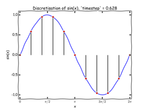
To solve these equations numerically we have to discretise the problem: rather than treating the atomic positions, velocities, and forces as continuous functions of time, we break our simulation up into a sequence of timesteps, each of length $\delta t$. This process is illustrated for a simple function in figure 1. The method that we are going to use to solve Newton's law for our atoms is usually called the Verlet algorithm (although it is an old method, and has been 'rediscovered' many times!). To understand its origin, we will begin with a brief derivation.

Figure 1: Discretisation of sin(x) between 0 and $2\pi$

We denote the position of an atom, $i$, at time $t$ by ${\mathbf{x}}_i\left(t\right)$. Similarly, ${\mathbf{v}}_i\left(t\right)$ is the velocity of that atom at the same time. What we want to know is the position of the atoms at the next timestep, $t+\delta t$. The basic Verlet algorithm is shown in figure 2 - knowing a set of initial conditions the algorithm calculates forces and by Newton's second law, we can update the positions of a set of particles are a time $t+\delta t$.

Figure 2: Steps to implement the classic Verlet algorithm.

TASK 1: By taking Taylor expansions of $x(t+\delta t)$ and $x(t-\delta t)$, write general expressions for them up to the fourth order ${𝒪}\left(\delta t^4\right)$

Having written these expressions, derive the formula in figure 2 to update positions as used in the classical Verlet algorithm $x(t+\delta t)\approx 2x_i(t)-x_i(t-\delta t)+\frac{F_i(t)}{m}\delta t^2$ by using Newton's second law to replace $\frac{{\mathrm{d}}^2{\mathbf{x}}_i\left(t\right)}{\mathrm{d}{t}^2}$ [4 marks]

Using this last equation, we can use a sequence of steps like those shown in figure 2 to get the positions. At no point are the velocities calculated in this method!

Velocity Verlet Algorithm

If we assume that the acceleration of an atom depends only on its position and not its velocity, then we are able to come up with a new algorithm that lets us calculate atomic velocities explicitly as shown in figure 3.

Figure 3: Steps to implement the velocity Verlet algorithm.

We start by noting that

$$\begin{gathered} {\mathbf{v}}_i(t+\delta t)={\mathbf{v}}_i\left(t\right)+\frac{{\mathbf{a}}_i\left(t\right)+{\mathbf{a}}_i(t+\delta t)}{2}\delta t \\ (6) \end{gathered}$$

We can Taylor expand the velocity by half a step, instead of a full step.

$$\begin{gathered} {\mathbf{v}}_i(t+\frac{1}{2}\delta t)={\mathbf{v}}_i\left(t\right)+\frac{1}{2}{\mathbf{a}}_i\left(t\right)\delta t \\ (7) \end{gathered}$$

We then substitute this into your expansion for $x_i(t+\delta t)$ to obtain an accuracy up to $\delta t^2$. Notice that terms up to $\delta t^2$ in your expansion can be written:

${\mathbf{x}}_i(t+\delta t)={\mathbf{x}}_i(t)+\mathbf{v}(t)\delta t+\frac{1}{2}\mathbf{a}(t)\delta t^2$

$$\begin{gathered} {\mathbf{x}}_i(t+\delta t)={\mathbf{x}}_i\left(t\right)+{\mathbf{v}}_i(t+\frac{1}{2}\delta t)\delta t \\ (8) \end{gathered}$$

When we know the updated atomic positions, we can calculate new forces, ${\mathbf{a}}_i(t+\delta t)$. Finally, we substitute equation (7) into equation (6) to get the new velocities ${\mathbf{v}}_i(t+\delta t)$.

$$\begin{gathered} {\mathbf{v}}_i(t+\delta t)={\mathbf{v}}_i(t+\frac{1}{2}\delta t)+\frac{1}{2}{\mathbf{a}}_i(t+\delta t)\delta t \\ (9) \end{gathered}$$

Notice that for both numerical integration algorithms, the first step is "specify initial conditions". When using the Verlet algorithm, we need to know the starting positions of the atoms (${\mathbf{x}}_i\left(0\right)$), and their positions one timestep in the past (${\mathbf{x}}_i(-\delta t)$). If the velocity-Verlet algorithm is used, then we have to know the the starting positions of the atoms (${\mathbf{x}}_i\left(0\right)$) and their velocities at the same time (${\mathbf{v}}_i\left(0\right)$). For this reason, we often start new simulations by using the output of older ones. If, however, you are performing your first simulations of a system (as we are now), then you must choose your initial conditions. The simulation software that we will use is able to do this for us, and this will be explained in the next section.

TASK 2: What could be an advantage of the Velocity-Verlet algorithm over the classical Verlet algorithm? [2 marks]

Atomic Forces

Since we can't reasonably solve the exact equations from quantum mechanics necessary to determine the forces acting on a given configuration of N atoms, we have to make approximations. We know from classical physics that the force acting on an object is determined by the potential that it experiences:

${\mathbf{F}}_i=-\frac{\mathrm{d}U\left({\mathbf{r}}^N\right)}{\mathrm{d}{\mathbf{r}}_i}$

The shorthand notation ${\mathbf{r}}^N$ stands for the position vectors of every atom in system. In principle, the force that a single atom feels is determined by the position of every other atom in the simulation. All we then need to do is to find a function $U$, the potential energy, that captures all the key physics of the interatomic interactions in the system. For many simple liquids, it turns out that we can model the interactions between each pair of atoms extremely well using the Lennard-Jones potential. Overall, U takes the form:

$$\begin{gathered} U\left({\mathbf{r}}^N\right)=\sum _{i=1}^{N-1}\sum _{j>i}^N\left\{4ϵ(\frac{{\sigma }^{12}}{r_{ij}^{12}}-\frac{{\sigma }^6}{r_{ij}^6})\right\} \\ (10) \end{gathered}$$

TASK 3: Consider the Lennard-Jones pair potential. What physical interaction(s) does it describe? What is the physical significance for the r^(-6) and r^(-12) terms? [3 marks]

TASK 4: For a single Lennard-Jones interaction, $\varphi \left(r\right)=4ϵ(\frac{{\sigma }^{12}}{r^{12}}-\frac{{\sigma }^6}{r^6})$, find the separation, $r_0$, at which the potential energy is zero. What is the force at this separation? Find the equilibrium separation, $r_{eq}$, and work out the well depth ($\varphi \left(r_{eq}\right)$). Evaluate the integrals $\underset{2\sigma }{\overset{\mathrm{\infty }}{\int }}\varphi \left(r\right)\mathrm{d}r$, $\underset{2.5\sigma }{\overset{\mathrm{\infty }}{\int }}\varphi \left(r\right)\mathrm{d}r$, and $\underset{3\sigma }{\overset{\mathrm{\infty }}{\int }}\varphi \left(r\right)\mathrm{d}r$ when $\sigma =ϵ=1.0$ [4 marks].

Periodic Boundary Conditions

Figure 4: Diagram of a simulation box containing 2139 atoms. The blue lines indicate the boundaries of the box.

Figure 5: Periodic boundary conditions in two dimensions.

We cannot simulate realistic volumes of liquid. In fact, in our simulations, $N$ will be between $1000$ and $10000$. The following task should illustrate why this must be so.

In order for our simulations to approximate a bulk liquid, we have to use a computational trick. The atoms in the simulation are enclosed in a simulation box, of fixed dimensions (figure 4). This box is very often a cuboid, but parallelepipeds can also be used (and this can be very useful when simulating crystal structures). We pretend that we have repeated our box infinitely in all directions, so that the atoms at the very edges are not exposed to a vacuum. This is illustrated in two dimensions in figure 5. The darker coloured atoms in the central box are the "real" atoms. The faded atoms in the outer four boxes are the replicas. When an atom crosses the boundary of the box, one of its replicas enters the box through the opposite face. In this way, the number of atoms inside the box is always constant.

TASK 5: Consider an atom at position $(0.5,0.5,0.5)$ in a cubic simulation box which runs from $(0,0,0)$ to $(1,1,1)$. In a single timestep, it moves along the vector $(0.7,0.6,0.2)$. At what point does it end up, after the periodic boundary conditions have been applied? [1 marks] .

Truncation

Periodic boundary conditions introduce their own problems. When we defined our potential function (equation 10), we specified that it depended on all possible pairs of atoms. If we have an infinite number of replicas of our system, how can we avoid calculating an infinite number of pair interactions?

Think about the three integrals you calculated for the Lennard-Jones potential task. They represent the area under the Lennard-Jones potential curve between some specified distance ($2\sigma$, $2.5\sigma$, and $3\sigma$), and infinite separation (where there is no interaction). You should find that this value becomes rather small as the near distance is increased! The attractive $\frac{1}{r^6}$ part of the potential dominates here, and this decays rapidly with $r$. We assume that this means that there is a distance beyond which the interaction is so small that we can safely ignore it. In fact, in most simulations this is chosen to be something close to $2.5\sigma$ or $3\sigma$. When the forces are calculated, we only calculate interactions between a pair of atoms if their separation is less than this cutoff.

Reduced Units

It is typical when using Lennard-Jones interactions to work in reduced units. By this, we mean that all quantities in our simulation are divided by scaling factors — for example, distances are divided by $\sigma$. The result of this is that the values become more manageable: all values that we might work out are typically around 1, rather than $1\times 10^{-10}$ (in the case of distance), $300$ (in the case of temperature), or $1\times 10^{-19}$ (in the case of energy).

We denote these reduced quantities by a star, and they take the following conversion factors:

• distance $r^{*}=\frac{r}{\sigma }$
• energy $E^{*}=\frac{E}{ϵ}$
• temperature $T^{*}=\frac{k_{B}T}{ϵ}$

TASK 6: The Lennard-Jones parameters for argon are $$\begin{gathered} \sigma =0.34\mathrm{n}\mathrm{m},ϵ \\ / \\ {k}_B=120\mathrm{K} \end{gathered}$$. If the LJ cutoff is $r^{*}=3.2$, what is it in real units? What is the well depth in $$\begin{gathered} {\mathrm{k}\mathrm{J} \\ \mathrm{m}\mathrm{o}\mathrm{l}}^{-1} \end{gathered}$$? What is the reduced temperature $T^{*}=1.5$ in real units? [1 marks]

This is the second section of the third year simulation experiment. You can return to the previous section, Files to Download, or jump ahead to the next section, Equilibration.