Talk:Mod:EnriqueLiquidsReport

Nice report - most things are explained well, your writing is direct and clear. Ensure you maintain a theme (especially for your MSci/BSc project) and tie everything back to that theme! Mark: 70/100

Report

Abstract

Molecular dynamics simulation was used to attempt to model a simple liquid and predict how its density and heat capacity varied with temperature using a Lennard-Jones potential, where both showed an decrease with temperature. The radial distribution function and diffusion coefficients were then also calculated at each phase in order to further investigate the structure, where an increase in disorder was seen going from solid to gas. It was subsequently concluded that the simulation was a success as the model behaved as expected on all counts.Well the lab wasn't as much about the simulation as it was about calculating the diffusion and dynamic properties with simulation - so these should be your ultimate conclusion. Also nice to include data in an abstract.

Introduction

Molecular dynamics simulation is a form of computational chemistry that allows us to investigate the physical motion of groups of particles as well as infer their physical properties. These include being able to determine a systems gram total energy, heat capacity, density and trajectories based on what potential function we specify for the system. The method can prove extremely useful as, once set up correctly, it allows us to predict how a given system may behave under certain conditions without having to setup an physical experiment. true, computational work is better than experimental work in every regard. :^)

In particular, molecular dynamics has found significant success in modelling the behaviour of proteins by helping to investigate their folding processes and their biological activity.Because the function of a protein heavily depends on its structural arrangement, understanding how a protein arranges itself under different conditions (such as at high or low PH) has proved crucial in determining how a protein may behave inside an organism. Whilst this can be partially investigated via the use of techniques such as X-Ray crystallography, this approach is time consuming and only provides one specific arrangement of our protein which may not always apply depending on what conditions our protein is subjected to. Thanks to molecular dynamics however, it is now possible to probe this initial structure further by applying different conditions to the protein and observing in real time how it rearranges itself, making it easier to predict how it may behave. One example of this methods success includes allowing researchers to characterise the catalytic function of complex enzymes such as Dihydrofolate reductase, giving a significant insight into its reaction kinetics and the flexibility of the enzyme's active site. It is clear that approaches like this wouldn't be possible without the use of molecular dynamics. although interesting, would be nice to see something related to states of matter - something like measurement of mobility by solid-state proton NMR in a system where immobility allows for the formation of deposits and phase heterogeneity. That would be something we could use in an introduction because, not only is it related to phase separation, this research was performed in a combustion chamber i.e. temperature dependent mobility and thus deposit formation dependence on temperature (dynamics varying with a thermodynamic property - a key underlying theme of this work). https://doi.org/10.4271/932811

Aims and objectives

Nice but could be written more concisely in bullet points- just an idea for your MSci proj.

Based on these principles, this experiment aimed to determine the dynamic and structural properties of a simple liquid as its physical properties were varied. These included investigating the density of the system as a function of temperature, the variation in heat capacity with temperature, the change in its radial distribution function and also determining the Diffusion coefficient of the system for the solid, liquid and gas phases using two different methods. All of this was done by using the program LAMMPS which was developed specifically for this purpose.

Methods

not a bad attempt - you introduce the software, the model. For the forcefield you must include information about cutoff too.

In order to simulate a simple liquid, the simulations were performed in LAMMPS using a lennard-jones potential with well depth ($ϵ$) and zero-potential length ($\sigma$) of 1.0 each in reduced units. One particle type of mass 1.0 was also used throughout the simulation .

A simple cubic lattice of number density 0.8 with dimensions of 15 x 15 x 15 unit cells was then melted under a specified temperature and pressure in order to form the desired state using an NVE ensemble. The particles were then assigned a random velocity such that the Maxwell-Boltzman *Boltzmann distribution was preserved for the simulation. tick

The variation in density was then calculated from the simulation using a range of given temperatures (T* = 2, 2.2, 2.4, 2.6, 2.8 ) and pressures (P* = 2.5, 3 ) in reduced units by switching to an NPT ensemble in order to allow *controlled* variation of these quantities. Likewise, the Heat capacities were then calculated by using the same range of temperatures but also two densities ( ρ* = 0.2 , 0.8) using an NVT ensemble. The radial distribution function was then determined for the solid (T*= 1 , ρ*= 1.2, fcc), liquid (T*= 1.2 ,  ρ*= 0.8) and gas (T*= 0.9 ,  ρ*= 0.05) phases in order to illustrate the structure of the system by using another program called VMD. Finally, the diffusion coefficients were calculated using the mean squared deviation (MSD) and the velocity auto-correlation function (VACF) of the system.

Results and Discussion

Number density as a function of temperature

Figure 1: Variation of Density with Temperature ( T = 2,4,6,8,10 ) at P = 2.5 and P = 3. The ideal gas law is also plotted for each case.

Figure 1 shows the variation of the number density with temperature for our simulation compared to the values predicted by the ideal gas law. A clear trend is seen where the density decreases with temperature. This occurs due to the increased amount of kinetic energy our particles posses at higher temperatures, allowing our particles to vibrate more hence take up a greater volume.

The predicted density generated from the ideal gas law is also higher than the actual densities we obtained. This occurs because the ideal gas law assumes that our particles don't interact at all except via elastic collisions, which causes the predicted densities to be much higher than our model's densities as the ideal gas law neglects to account for the repulsive interactions felt by the particles as they get close to each other (and hence reducing the number of particles per unit volume). In comparison, our simulation accounts for this by using the lennard-jones equation. Additionally, this discrepancy increases with pressure as our particles are being forced closer to each other and so experience a larger repulsive force, causing a reduction in the number of particles per unit volume as a result. tick, good. What about the behaviour of our system at high T?

Heat capacity as a function of temperature

Figure 2: Plot of heat capacity (divided by volume) against temperature at densities of 0.2 and 0.8.

The heat capacity of our substance appears to decrease with temperature as shown in figure 2. This occurs as expected because as our molecules reach a higher temperature, there is a higher density of states in the excited region of our system. This makes it easier to heat our system at higher Temperatures due to the atomic energy gaps decreasing in size as we excite the molecule further. nice

In addition, heat capacity also appears to increase with density. This makes sense because at a higher density, our system has more atoms present per unit volume hence more energy levels that must be excited before an increase in temperature is seen. This means we now require more energy to excite our system to the next energy level in order to raise the temperature. good

Additionally, a slight hump can be seen in the 0.8 density case. This is due to the system changing phase, causing it to gain a large influx of degrees of freedom which now contribute to the heat capacity, raising it.tick

Radial distribution function

Figure 3: Plots of the radial distribution function and its associated integral as a function of radius for the solid, liquid and gas phases.

Figure 3 shows the Radial gram distribution function and its associated integral for the solid, liquid and gas phases of our substance. Compared to the liquid and gas phases, the solid RDF contains significantly more maxima and it decays to one much more slowly compared to the other two phases. This occurs because in the solid phase, our atoms have a regular/periodic structure where our atoms are held roughly in the same place (but can undergo some vibrational movement). As a result we see a number of peaks in our RDF which represent the different coordination shells that surround our reference particle. Our function also decays to one (corresponding to the bulk density of our substance) much more slowly than the other phases due to the long range lattice structure the atoms in our solid have. tick

The liquid phase and gas phases in comparison have fewer maxima and decay much more quickly. This occurs because our atoms passive tone! are not fixed in one position and are able to move around more easily, which causes them to lose their long range structure. Compared to the gas phase, the liquid phase does still have an initial structure and exhibits coordination shells at short distances due to the attractive forces between our atoms at these distances. Whilst the gas phase does have a similar RDF to our liquid, it decays to one even quicker and only has one significant maximum. Again, our atoms have very little structure and are more dispersed than our liquid phase, causing them to feel less attractive force between each other. tick, good

We can also infer the appearance of the coordination shells for our phases by looking at the running integral for each phase and comparing it to the peaks seen in our RDF. This is particularly useful for the solid RDF as the first three maxima correspond to the three initial coordination shells of the FCC lattice, consisting of 12, 6 and 24 atoms respectively. These have been illustrated in figure 4:

Figure 4: Diagram showing the first, second and third coordination shells of the solid phase from left to right.

tick

Mean squared displacement

Figure 5: Plots of the Mean squared displacement as a function of timestep for the solid, liquid and gas phases of our simulation.

Table 1: Calculated diffusion coefficients from the MSD for 1000 and 1,000,000 atom systems.

Number of atoms	Solid diffusion coefficient	Liquid diffusion coefficient	Gas diffusion coefficient
1000	-1.17 x 10-7 m2 / s	0.0849 m2 / s	2.19 m2 / s
1,000,000	-8.33 x 10-6 m2 / s	0.0873 m2 / s	3.02 m2 / s

Figure 5 shows the Mean squared displacement gram for each phase of our simulation, appearing as expected for all our phases. For the solid phase the atoms are fixed in position and can vibrate, but are unable to diffuse significantly from their lattice structure. This is reflected by it's oscillating MSD , which shows our atoms are at roughly the same distance from our reference position as time goes on. In the liquid and gas cases, our atoms are no longer fixed in position and are able to diffuse through our system (the gas does this the most as it has the lowest amount of interactions between its atoms). This explains the linear increase in the MSD as time goes on as our atoms are diffusing further from our initial position. Linear why? Linear because msd and time have a linear relationship (power law) in the diffusive regime.

The diffusion coefficients were then calculated by using the equation: $D=\frac{1}{6}\frac{\partial ⟨r^2\left(t\right)⟩}{\partial t}$ . Table 1 shows the results of our simulation in comparison to a 1,000,000 atom system. These results suggest our simulation has been successful in modelling a simple liquid as our diffusion coefficients increase as we go from the solid to gas phase. Our values also compare well to that of the larger system. tick

Velocity auto-correlation function

Figure 6: Plot of our VACF and its running integrals for each phase of our simulation against time. The 1D harmonic oscillator has also has its VACF plotted for comparison.

Table 2: Calculated diffusion coefficients from the VACF for 1000 and 1,000,000 atom systems.

Number of atoms	Solid diffusion coefficient	Liquid diffusion coefficient	Gas diffusion coefficient
1000	1.88 x 10-4 m2 / s	0.0979 m2 / s	2.37 m2 / s
1,000,000	4.55 x 10-5 m2 / s	0.0901 m2 / s	3.27 m2 / s

The VACF are shown for each phase in figure 6 along with the 1D harmonic oscillator VACF for comparison, which was determined using the relation: $C\left(\tau \right)=\frac{\underset{-\mathrm{\infty }}{\overset{\mathrm{\infty }}{\int }}{\omega }^2{A}^2\sin (\omega t+\varphi )\sin (\omega (t+\tau )+\varphi )\mathrm{d}t}{\underset{-\mathrm{\infty }}{\overset{\mathrm{\infty }}{\int }}(-\omega A\sin (\omega t+\varphi ){)}^2\mathrm{d}t}=\cos (\omega \tau )$.

Again, the VACF appear as expected for each phase of our simulation. Compared to the gas phase, the solid and liquid cases contain minima which are produced due to the strong interactions that the atoms feel between each other as they travel through the system. These indicate that the atoms have reversed their velocity and are travelling in the opposite direction to their initial velocity. you're alluding to the right answer but haven't quite hit the nail on the head. The first minima portray a picture of the collision dynamics in the system. Specifically, the first minimum gives the time at which all particles have collided at least once.

The liquid and solid VACF's also differ, with the liquid case decaying to zero more quickly and oscillating less than the solid. This is because in the solid phase, our atoms are packed closer together and have a fixed structure, so they experience a larger amount of attractive/repulsive forces as they attempt to move through the system. there are more initial collisions! This results in the VACF oscillating more strongly as our atoms velocities are still correlated due to the fixed structure they exist in. In the liquid phase, our atoms don't have a fixed structure and undergo diffusion much more readily, which causes the velocities of our atoms to be less correlated.

The solid and liquid phases also differ compared to the harmonic VACF function, which doesn't appear to decay in time. Notably, the harmonic oscillator assumes our atoms don't lose energy, causing our atoms velocities to oscillate in an undamped SHM pattern. This neglects any other attractive/repulsive interactions that occur in the system (unlike our simulation where this is accounted for) which would result in a decay in our VACF. tick, good

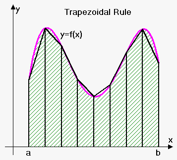
The calculated diffusion coefficients are also shown in table 2 compared to our 1,000,000 atom case again. These were obtained using the Trapezium rule along with the relation: $D=\frac{1}{3}\underset{0}{\overset{\mathrm{\infty }}{\int }}\mathrm{d}\tau ⟨\mathbf{v}\left(0\right)\cdot \mathbf{v}\left(\tau \right)⟩$. Once again, our diffusion coefficients match well with theory and compare favourably to the larger system using this method. There is still some deviation in our values however, which likely comes from the trapezium rule itself as it will often under/over estimate or our integral due to how it overlaps with the line we have plotted. An example of this is shown in figure 7.tick

Figure 7: Diagram showing how the trapezium rule will underestimate or overestimate a function based on whether the function approaches a maxima or minima respectively. Taken from

Conclusion

In summary, a simple liquid was successfully simulated using the LAMMPS program based on a Lennard-Jones potential in order to determine how its density and heat capacity varied with temperature. These were both found to decrease with temperature as expected due to the increased kinetic energy of the particles and the decreasing energy gap as the liquid is heated respectively. The RDF and diffusion coefficients were also calculated for each phase and appeared in accordance with the structural features of each phase, with the solid phase having the slowest decaying RDF and smallest diffusion coefficient due to its more organised fixed lattice structure. In comparison, the liquid and gas phases saw the opposite occur due to their increasingly dispersed and disorganised structures.

Tasks / Lab book

TASK: Open the file HO.xls.

In it, the velocity-Verlet algorithm is used to model the behaviour of a classical harmonic oscillator. Complete the three columns "ANALYTICAL", "ERROR", and "ENERGY": "ANALYTICAL" should contain the value of the classical solution for the position at time $t$, "ERROR" should contain the absolute difference between "ANALYTICAL" and the velocity-Verlet solution (i.e. ERROR should always be positive -- make sure you leave the half step rows blank!), and "ENERGY" should contain the total energy of the oscillator for the velocity-Verlet solution. Remember that the position of a classical harmonic oscillator is given by $x\left(t\right)=A\cos (\omega t+\varphi )$ (the values of $A$, $\omega$, and $\varphi$ are worked out for you in the sheet).

TASK: For the default timestep value, 0.1, estimate the positions of the maxima in the ERROR column as a function of time. Make a plot showing these values as a function of time, and fit an appropriate function to the data.

would be nice to see your linear fit on superposed on error

Media:HO_EJR15.xls

TASK: Experiment with different values of the timestep. What sort of a timestep do you need to use to ensure that the total energy does not change by more than 1% over the course of your "simulation"? Why do you think it is important to monitor the total energy of a physical system when modelling its behaviour numerically?

0.25 timestep works quite well, giving 4.96e-1 average which stays within 1% on either side. We should monitor the energy of our system when modelling its behavior numerically as if the energy changes too much from the real value our calculations may be invalid for our system (it should be as close to the real life energy as possible in order for our system to be accurate). I would argue that 0.25 doesn't work well enough - the spread is still a little too large.

TASK: For a single Lennard-Jones interaction,

$\varphi \left(r\right)=4ϵ(\frac{{\sigma }^{12}}{r^{12}}-\frac{{\sigma }^6}{r^6})$, find the separation, $r_0$, at which the potential energy is zero.

$r_0=\sigma$

What is the force at this separation?

$\frac{24ϵ}{r{0}_{}}$tick

Find the equilibrium separation, $r_{eq}$, and work out the well depth ($\varphi \left(r_{eq}\right)$).

$r_{eq}=\sqrt[6]{2r^6}$ and $\varphi \left(r_{eq}\right)=-ϵ$tick

Evaluate the integrals $\underset{2\sigma }{\overset{\mathrm{\infty }}{\int }}\varphi \left(r\right)\mathrm{d}r$, $\underset{2.5\sigma }{\overset{\mathrm{\infty }}{\int }}\varphi \left(r\right)\mathrm{d}r$, and $\underset{3\sigma }{\overset{\mathrm{\infty }}{\int }}\varphi \left(r\right)\mathrm{d}r$ when $\sigma =ϵ=1.0$.

$\underset{2\sigma }{\overset{\mathrm{\infty }}{\int }}\varphi \left(r\right)\mathrm{d}r=-0.0248$tick

$\underset{2.5\sigma }{\overset{\mathrm{\infty }}{\int }}\varphi \left(r\right)\mathrm{d}r=-8.178\times 10^{-3}$tick

$\underset{3\sigma }{\overset{\mathrm{\infty }}{\int }}\varphi \left(r\right)\mathrm{d}r=-3.29\times 10^{-3}$tick

TASK: Estimate the number of water molecules in 1ml of water under standard conditions.

Estimate the volume of  10,000 water molecules under standard conditions.

1 ml is roughly 1g of water. Using this fact, we can calculate the moles of water in 1ml by doing 1/18 = 0.0556 moles of water. We can then multiply by Avogadro's number (6.022e22) to get 3.345e22 molecules of water. tick

The volume of 10,000 water molecules is obtained by dividing by avogadro's number to get 1.661e-20 moles of water. You can then multiply this by the molecular weight (which is 18 in this case) to get a mass of 2.989e-19 g. Finally, since 1g of water is roughly 1 ml, we can say the volume of 10,000 molecules of water is 2.989e-19 mltick

TASK: Consider an atom at position

$(0.5,0.5,0.5)$ in a cubic simulation box which runs from $(0,0,0)$ to $(1,1,1)$. In a single timestep, it moves along the vector $(0.7,0.6,0.2)$. At what point does it end up, after the periodic boundary conditions have been applied?.

$(0.5,0.5,0.5)+(0.7,0.6,0.2)=(0.2,0.1,0.7)$ tick

TASK: The Lennard-Jones parameters for argon

are $$\begin{gathered} \sigma =0.34\mathrm{n}\mathrm{m},ϵ \\ / \\ {k}_B=120\mathrm{K} \end{gathered}$$. If the LJ cutoff is $r^{*}=3.2$, what is it in real units? What is the well depth in $$\begin{gathered} {\mathrm{k}\mathrm{J} \\ \mathrm{m}\mathrm{o}\mathrm{l}}^{-1} \end{gathered}$$? What is the reduced temperature $T^{*}=1.5$ in real units?

$r=1.088\mathrm{n}\mathrm{m}$

$ϵ=0.998KJmo{l}^{-1}$

$T=180K$ tick

TASK: Why do you think giving atoms random starting coordinates causes problems in simulations?

Hint: what happens if two atoms happen to be generated close together?

If two atoms happen to be generated close to each other via this method, they will experience *they can experience if placed to close to each other a strong interaction as determined by the lennard-jones equation. This may make it difficult for the system to reach equilibrium due to these interactions.

TASK: Satisfy yourself that this lattice spacing corresponds to a number density of lattice points of . Consider instead a face-centred cubic lattice with a lattice point number density of 1.2. What is the side length of the cubic unit cell?

$p=\frac{m}{v}$

$\frac{1}{1.07722^3}=0.8$ tick

For fcc:

$L=\sqrt[3]{\frac{4}{1.2}}=1.494$tick

TASK: Consider again the face-centred cubic lattice from the previous task.

How many atoms would be created by the create_atoms command if you had defined that lattice instead?

For a 10x10x10 box, you should have 4000 atoms

TASK: Using the LAMMPS manual, find the purpose of the following commands in the input script:

mass 1 1.0
pair_style lj/cut 3.0
pair_coeff * * 1.0 1.0

Mass 1 1.0 sets the mass of atom type 1 to 1.0 grams.

pair_style sets the formula we use to compute pairwise interactions. In our case we've picked a lennard-jones potential with a cuttoff value of r = 3.

pair_coeff defines our forcefield coefficients for the atom pair types we've defined. In the case of lennard-jones, our coefficients include the well depth and the zero potential distance.

TASK: Given that we are specifying ${\mathbf{x}}_i\left(0\right)$ and ${\mathbf{v}}_i\left(0\right)$, which integration algorithm are we going to use?

The velocity-Verlet algorithm

TASK: Look at the lines below.

### SPECIFY TIMESTEP ###
variable timestep equal 0.001
variable n_steps equal floor(100/${timestep})
timestep ${timestep}

### RUN SIMULATION ###
run ${n_steps}
run 100000

The second line (starting "variable timestep...") tells LAMMPS that if it encounters the text ${timestep} on a subsequent line, it should replace it by the value given. In this case, the value ${timestep} is always replaced by 0.001. In light of this, what do you think the purpose of these lines is? Why not just write:

timestep 0.001
run 100000

Ask the demonstrator if you need help.

By using a variable, we can easily change our value for the timestep in our script by just modifying this variable's value. This will change the timestep value for all parts of the script that use it easily. It also allows us to change timesteps/modify them easily.

TASK: make plots of the energy, temperature, and pressure, against time for the 0.001 timestep experiment (attach a picture to your report).

Does the simulation reach equilibrium? How long does this take? When you have done this, make a single plot which shows the energy versus time for all of the timesteps (again, attach a picture to your report). Choosing a timestep is a balancing act: the shorter the timestep, the more accurately the results of your simulation will reflect the physical reality; short timesteps, however, mean that the same number of simulation steps cover a shorter amount of actual time, and this is very unhelpful if the process you want to study requires observation over a long time. Of the five timesteps that you used, which is the largest to give acceptable results? Which one of the five is a particularly bad choice? Why?

Plots of temperature, Pressure and Total energy over time for the 0.001 time step selected.

Ensure your scaling is nice on your graphs (your 0.015 divergence cuts off the top.

Plot of all time steps showing change in total energy over time.

The 0.001 time step reaches equilibrium very quickly in around 2 seconds. Compared to the other 4 timesteps, the 0.0025 time step also reaches equilibrium in around the same time however the same cannot be said for the others. The worst choice of time step would be the 0.015 time step in this case, as instead of tending towards an equilibrium amount of energy it is instead increasing in energy. This indicates our calculations may be inaccurate compared to how the experiment would behave in real life. tick

TASK: Choose 5 temperatures (above the critical temperature $T^{*}=1.5$), and two pressures

(you can get a good idea of what a reasonable pressure is in Lennard-Jones units by looking at the average pressure of your simulations from the last section). This gives ten phase points — five temperatures at each pressure. Create 10 copies of npt.in, and modify each to run a simulation at one of your chosen $(p,T)$ points. You should be able to use the results of the previous section to choose a timestep. Submit these ten jobs to the HPC portal. While you wait for them to finish, you should read the next section.

TASK: We need to choose $\gamma$ so that the temperature is correct $T=\mathfrak{𝔗}$ if we multiply every velocity $\gamma$. We can write two equations:

$\frac{1}{2}\sum _i{m}_i{v}_i^2=\frac{3}{2}N{k}_{B}T$

$\frac{1}{2}\sum _i{m}_i{\left(\gamma v_i\right)}^2=\frac{3}{2}N{k}_B\mathfrak{𝔗}$

Solve these to determine $\gamma$

Divide the two equations as shown:

$\frac{\frac{1}{2}\sum _i{m}_i{v}_i^2=\frac{3}{2}N{k}_{B}T}{\frac{1}{2}\sum _i{m}_i{\left(\gamma v_i\right)}^2=\frac{3}{2}N{k}_B\mathfrak{𝔗}}$

Cancelling down gives: $\frac{1}{{\gamma }^2}=\frac{T}{\mathfrak{𝔗}}$

Taking the inverse and then the square root gives the final answer:

$\gamma =\sqrt{\frac{\mathfrak{𝔗}}{T}}$ tick

TASK: Use the manual page to find out the importance of the three numbers 100 1000 100000.

How often will values of the temperature, etc., be sampled for the average? How many measurements contribute to the average? Looking to the following line, how much time will you simulate?

The three numbers are used to assign 3 variables: Nevery, Nrepeat and Nfreq.

Nevery instructs lammps to take an sample of our data after a certain number of timesteps (in our case, 100).

Nrepeat then tells lammps to take an average of our now sampled data after a certain number of timesteps (in this case every 1000)

Finally, Nfreq tells lammps to calculate an final average of these previous averages after so many time steps (in our case, 100,000).

For this simulation, this is essentially a way of telling lammps to average our whole data set since we're running this simulation for 100,000 timesteps (which is 250 seconds for a 0.0025 timestep). Hence all our measurements are part of this final average. tick

TASK: When your simulations have finished, download the log files as before.

At the end of the log file, LAMMPS will output the values and errors for the pressure, temperature, and density $\left(\frac{N}{V}\right)$. Use software of your choice to plot the density as a function of temperature for both of the pressures that you simulated. Your graph(s) should include error bars in both the x and y directions. You should also include a line corresponding to the density predicted by the ideal gas law at that pressure. Is your simulated density lower or higher? Justify this. Does the discrepancy increase or decrease with pressure?

Variation of Density with Temperature ( T = 2,4,6,8,10 ) at P = 2.5 and P = 3. The ideal gas law is also plotted for each case.

The predicted density generated from the ideal gas law is higher than the actual densities we obtained. This occurs because the ideal gas law assumes that our particles don't interact at all except via elastic collisions. This causes the predicted densities to be much higher than our model's densities as the ideal gas law neglects to take into account the repulsive interactions felt by the particles as they get close to each other (and hence reducing the number of particles you can find per unit volume). In comparison, our model accounts for this by using the lennard-jones equation.

This discrepancy increases with pressure as our particles are being forced closer to each other and so experience a larger repulsive force, causing a reduction in the number of particles per unit volume as a result.

TASK: As in the last section, you need to run simulations at ten phase points.

In this section, we will be in density-temperature $({\rho }^{*},T^{*})$ phase space, rather than pressure-temperature phase space. The two densities required at $0.2$ and $0.8$, and the temperature range is $2.0,2.2,2.4,2.6,2.8$. Plot $C_V/V$ as a function of temperature, where $V$ is the volume of the simulation cell, for both of your densities (on the same graph). Is the trend the one you would expect? Attach an example of one of your input scripts to your report.

Plot of heat capacity (divided by volume) variation with temperature at densities of 0.2 and 0.8.

The heat capacity of our substance appears to decrease with temperature. This occurs as expected because as our molecules reach a higher temperature there is a higher density of states in the excited state region of our system. Because of this, it becomes easier to heat up our system at higher Temperatures due to the next atomic energy gap being much closer in energy to the previous energy gaps.

In addition the heat capacity also appears to increase with density. This makes sense because at a higher density, our system has more energy levels that require energy to be excited from. This means we now require more energy to excite our system to the next energy level and hence raise the temperature.

One example of an input script can be seen here: Media:P0.2t2.8 - volEJR15

TASK: perform simulations of the Lennard-Jones system in the three phases.

Plots of the radial distribution function and its associated integral as a function of radius for the solid, liquid and gas phases.

When each is complete, download the trajectory and calculate $g(r)$ and $\int g(r)\mathrm{d}r$. Plot the RDFs for the three systems on the same axes, and attach a copy to your report. Discuss qualitatively the differences between the three RDFs, and what this tells you about the structure of the system in each phase. In the solid case, illustrate which lattice sites the first three peaks correspond to. What is the lattice spacing? What is the coordination number for each of the first three peaks?

The Radial distribution function differs between the solid, liquid and gas phases of our substance in a few main ways. Compared to the liquid and gas phases, the solid RDF contains significantly more maxima and it also decays to one much more slowly compared to the other two phases. This occurs because in the solid phase, our atoms have a regular/periodic structure where our atoms are held roughly in the same place (but can undergo some vibrational movement). As a result we see a number of peaks in our RDF plot which represent the different coordination shells that surround our reference particle. Our function also decays to one (corresponding to the bulk density of our substance) much more slowly than the other phases due to the long range lattice structure the atoms in our solid have.

The liquid phase in comparison has fewer maxima and it's RDF decays much more quickly to one. This occurs because our atoms are not fixed in one position in the liquid phase and are instead able to move around more easily, which causes them to lose their long range structure quickly. This is shown by the RDF showing fewer peaks and more quickly decaying to one. However, the liquid phase does still have an initial structure and exhibits coordination shells at short distances (as seen by the first few peaks in the RDF) due to the attractive forces felt between our atoms at these distances.

The gas phase has a similar RDF to our liquid phase however it decays to one even more quickly and only really has one significant maximum. This occurs because in the gas phase our atoms essentially have very little structure and are significantly more dispersed than our liquid phase. As a result the atoms feel even less attractive force between each other, so much so that there is essentially only one coordination shell for the gas phase. After this point the atoms are much more diffuse and have no real structure, causing the RDF to quickly tend to the bulk density value.

The lattice spacing can be calculated from the density and number of lattice points in of our unit cell. By using the formula P=N/V with P=1.2 and N=4 (since we are using a fcc unit cell), our lattice spacing is therefore equal to 1.494.

Plot of the radial distribution function and the integrated radial distribution function for the solid phase.

The first 3 peaks in the solid RDF correspond to three coordination shells consisting of 12, 6 and 24 coordinating atoms respectively. These have been illustrated below.

Diagram showing the first, second and third coordination shells of the solid phase from left to right.

TASK: make a plot for each of your simulations (solid, liquid, and gas), showing the mean squared displacement (the "total" MSD) as a function of timestep.

Are these as you would expect? Estimate D in each case. Be careful with the units! Repeat this procedure for the MSD data that you were given from the one million atom simulations.

Plots of the Mean squared displacement as a function of timestep for the solid, liquid and gas phases of our simulation.

Gas diffusion coefficient = 2.19 m² / s

Solid diffusion coefficient = -1.17 x 10^-7 m² / s

Liquid diffusion coefficient = 0.0849 m² / s

One million atom system:

Plots of the Mean squared displacement as a function of timestep for the solid, liquid and gas phases of the 1,000,000 atom simulation.

Gas diffusion coefficient = 3.02 m² / s

Solid diffusion coefficient = -8.33 x 10^-6 m² / s

Liquid diffusion coefficient = 0.0873 m² / s

The Mean squared displacement behaves as expected for each phase. For our solid phase, the atoms are fixed in position and can vibrate, but are unable to diffuse significantly from their lattice structure. This is reflected by the oscillating line seen in it's MSD graph, which shows our atoms are at roughly the same distance from our reference position as time goes on. In the liquid and gas cases, our atoms are no longer fixed in position and are able to diffuse through our system with ease (the gas does this the most as it has the lowest amount of interactions between its atoms). This explains the linear increase in the MSD as time goes on as our atoms are diffusing further and further from our initial reference position.

TASK: In the theoretical section at the beginning, the equation for the evolution of the position of a 1D harmonic oscillator as a function of time was given.

Using this, evaluate the normalised velocity autocorrelation function for a 1D harmonic oscillator (it is analytic!):

$C\left(\tau \right)=\frac{\underset{-\mathrm{\infty }}{\overset{\mathrm{\infty }}{\int }}v\left(t\right)v(t+\tau )\mathrm{d}t}{\underset{-\mathrm{\infty }}{\overset{\mathrm{\infty }}{\int }}{v}^2\left(t\right)\mathrm{d}t}$

Be sure to show your working in your writeup.

First, we differentiate our equation for the 1D harmonic oscillator ($x\left(t\right)=A\cos (\omega t+\varphi )$) with respect to time to get:

$\frac{\partial x}{\partial t}=v\left(t\right)=-\omega A\sin (\omega t+\varphi )$

We then insert this into the normalised velocity autocorrelation function:

$C\left(\tau \right)=\frac{\underset{-\mathrm{\infty }}{\overset{\mathrm{\infty }}{\int }}{\omega }^2{A}^2\sin (\omega t+\varphi )\sin (\omega (t+\tau )+\varphi )\mathrm{d}t}{\underset{-\mathrm{\infty }}{\overset{\mathrm{\infty }}{\int }}(-\omega A\sin (\omega t+\varphi ){)}^2\mathrm{d}t}$

This can be further simplified by cancelling terms and expanding to give:

$C\left(\tau \right)=\frac{\underset{-\mathrm{\infty }}{\overset{\mathrm{\infty }}{\int }}\sin (\omega t+\varphi )\sin (\omega (t+\tau )+\varphi )\mathrm{d}t}{\underset{-\mathrm{\infty }}{\overset{\mathrm{\infty }}{\int }}{\sin }^2(\omega t+\varphi )\mathrm{d}t}$

The next step requires us to substitute in two trigonometric identities. The numerator requires us to use $\sin u\sin v=\frac{1}{2}[\cos (u-v)-\cos (u+v))]$

whilst the denominator requires the expression: $si{n}^{2}u=\frac{1-\cos (2u))}{2}$ .

Substituting these both in and cancelling the halves gives:

$C\left(\tau \right)=\frac{\underset{-\mathrm{\infty }}{\overset{\mathrm{\infty }}{\int }}\cos (-\omega \tau )-\cos (2\omega t+\omega \tau +2\varphi )\mathrm{d}t}{\underset{-\mathrm{\infty }}{\overset{\mathrm{\infty }}{\int }}1-\cos (2\omega t+2\varphi )\mathrm{d}t}$

We then integrate with respect to t:

$C\left(\tau \right)={\left[\frac{t\cos (-\omega \tau )-\frac{1}{2\omega }\sin (2\omega t+\omega \tau +2\varphi )}{t-\frac{1}{2\omega }\sin (2\omega t+2\varphi )}\right]}_{-\mathrm{\infty }}^{\mathrm{\infty }}$

In order to evaluate our expression successfully, we then divide the top and bottom by t:

$C\left(\tau \right)={\left[\frac{\cos (-\omega \tau )-\frac{1}{2\omega t}\sin (2\omega t+\omega \tau +2\varphi )}{1-\frac{1}{2\omega t}\sin (2\omega t+2\varphi )}\right]}_{-\mathrm{\infty }}^{\mathrm{\infty }}$

and calculate our interval. This gives us:

$C\left(\tau \right)=\frac{\cos (-\omega \tau )-0}{1-0}$

which can be simplified to $C\left(\tau \right)=\cos (\omega \tau )$

On the same graph, with x range 0 to 500, plot $C\left(\tau \right)$ with $\omega =1/2\pi$ and the VACFs from your liquid and solid simulations. What do the minima in the VACFs for the liquid and solid system represent? Discuss the origin of the differences between the liquid and solid VACFs. The harmonic oscillator VACF is very different to the Lennard Jones solid and liquid. Why is this? Attach a copy of your plot to your writeup.

Plot of VACF for the gas, liquid and solid phases of our simulation.

The minima in the VACF for the solid and liquid cases are produced due to the strong intermolecular interactions that the atoms feel between each other as they travel through the system. It indicates that the atom has reversed it's velocity and is travelling in the opposite direction to it's initial velocity.

The liquid and solid VACF's also differ, with the liquid case decaying to zero much more quickly and oscillating much less than the solid case. This is because in the solid phase, our atoms are packed much more closely together and have a fixed structure, so they experience a much larger amount of attractive/repulsive forces as they attempt to move through the system. As a result, the VACF oscillates strongly as our atoms velocities are still correlated due to the fixed structure they exist in. In the liquid phase, our atoms don't have a fixed structure (so experience less attractive/repulsive forces) and undergo diffusion much more readily. This causes our VACF function to oscillate less and decay to zero much more quickly as the velocities of our atoms are less correlated due to this diffusive motion and more disorganized structure.

Our harmonic VACF function doesn't appear to decay in time compared to the lennard-jones solid and liquid. This occurs because the harmonic oscillator assumes our atoms behave like two masses attached by a spring and assumes there is no loss of energy for our system, causing our atoms to oscillate via SHM (which is reflected in the velocity autocorrelation function). This approach neglects any other possible interactions that occur in the atom, for example interactions between the atom pair and any other nearby atoms in our system. When we account for this in our lennard-jones simulations, we see a notable decay in our velocity correlation function as time goes on due to the increasing number of interactions from other atoms as our reference atom moves through the system.

TASK: Use the trapezium rule to approximate the integral under the velocity autocorrelation function for the solid, liquid, and gas, and use these values to estimate $D$ in each case.

You should make a plot of the running integral in each case. Are they as you expect? Repeat this procedure for the VACF data that you were given from the one million atom simulations. What do you think is the largest source of error in your estimates of D from the VACF?

Plot of running VACF integrals for each phase of our simulation against time (left is our simulation, right is for the provided data for 1,000,00 atoms)

Simulation diffusion coefficients

Gas diffusion coefficient = 2.37 m² / s

Solid diffusion coefficient = 1.88 x 10^-4 m² / s

Liquid diffusion coefficient = 0.0979 m² / s

1,000,000 atoms diffusion coefficients

Gas diffusion coefficient = 3.27 m² / s

Solid diffusion coefficient = 4.55 x 10^-5 m² / s

Liquid diffusion coefficient = 0.0901 m² / s

Diagram showing how the trapezium rule will underestimate or overestimate a function based on whether the function approaches a maxima or minima respectively. Taken from: http://www.emathhelp.net/images/calc/322_trapezoidal_rule.png

The largest source of error in our diffusion coefficient comes from the trapezium rule itself, as it will often underestimate or overestimate our integral due to how it overlaps with the line we have plotted. This is then incorporated into our diffusion coefficient.

References

- ↑ D. C. Rapaport and D. C., The art of molecular dynamics simulation, Cambridge University Press, 1995.
- ↑ M. Karplus and J. Kuriyan, Proc. Natl. Acad. Sci. U. S. A., 2005, 102, 6679–85.
- ↑ C. O. Tomas Hansson and W. F. van Gunsteren*, Curr. Opin. Struct. Biol., 2002, 12, 190–196.
- ↑ J. R. Schnell, H. J. Dyson and P. E. Wright, Annu. Rev. Biophys. Biomol. Struct., 2004, 33, 119–140.
- ↑ http://lammps.sandia.gov
- ↑ J.-P. Hansen and L. Verlet, Phys. Rev., 1969, 184, 151–161.
- ↑ http://www.ks.uiuc.edu/Research/vmd/
- ↑ P. Atkins and J. De Paula, Atkins’ Physical chemistry 9th edition, 2009.
- ↑ J. Cohn, J. Phys. Chem., 1968, 72, 608–616.
- ↑ http://www.emathhelp.net/images/calc/322_trapezoidal_rule.png