Rep:Mod:xl3209module3

Third Year Computational Project- Module 3, Physical chemistry, Xizhou Liu, CID: 00593697

Introduction

1 hartree = 627.509 kcal mol^-1 To extend the scope of computational analysis from vibrational analysis , molecular orbitals and natural bond orbital analysis, in this module, computational analysis is used in discovering the transition states. Force Constant Matrix, Frozen Coordinate and QST2 methods are implemented with AM1, HF and DFT levels of theories. Furthermore the IRC path built in gaussian enables to follow the reaction path from transition state to the product.

The Cope Rearrangement

Introduction

Figure 1. The Cope Rearrangement Mechanism and two TS Conformers

The Cope Rearrangement reaction has been long established as a pericyclic reaction ([3,3]-sigmatropic shifts). However its reaction mechanism remains a controversial topic. The concerted rearrangement reaction is considered to have two different possible transition state, either the aromatic transition state or the diradical transition state. The aromatic transition state is shown in Figure 1 and has two conformations: the chair and the boat.

In order to study the rearrangement mechanisms, the reactant, product and transition states were optimized and further interpreted in two different levels of theory (HF and DFT).

Reactants and Products

Optimization

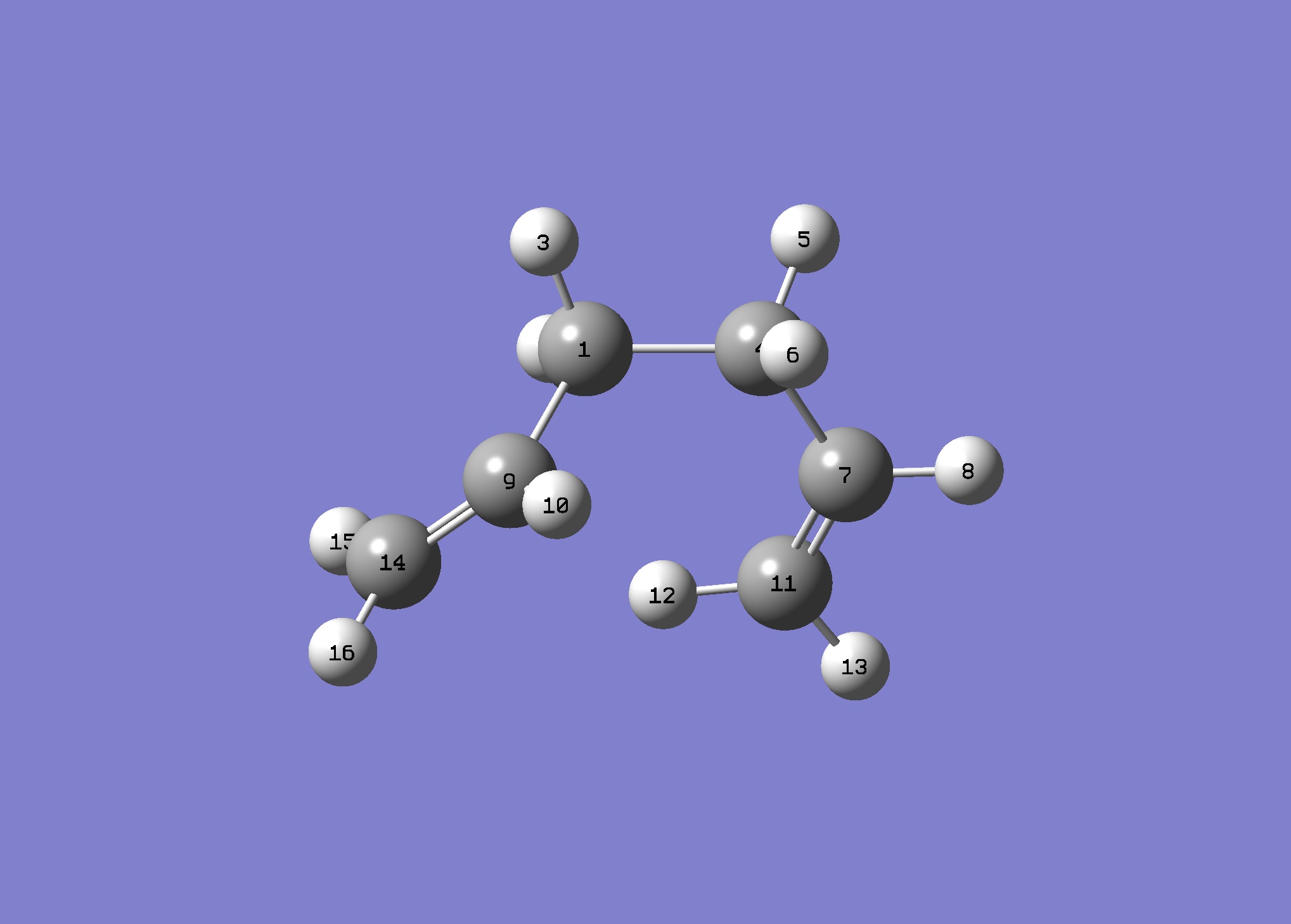
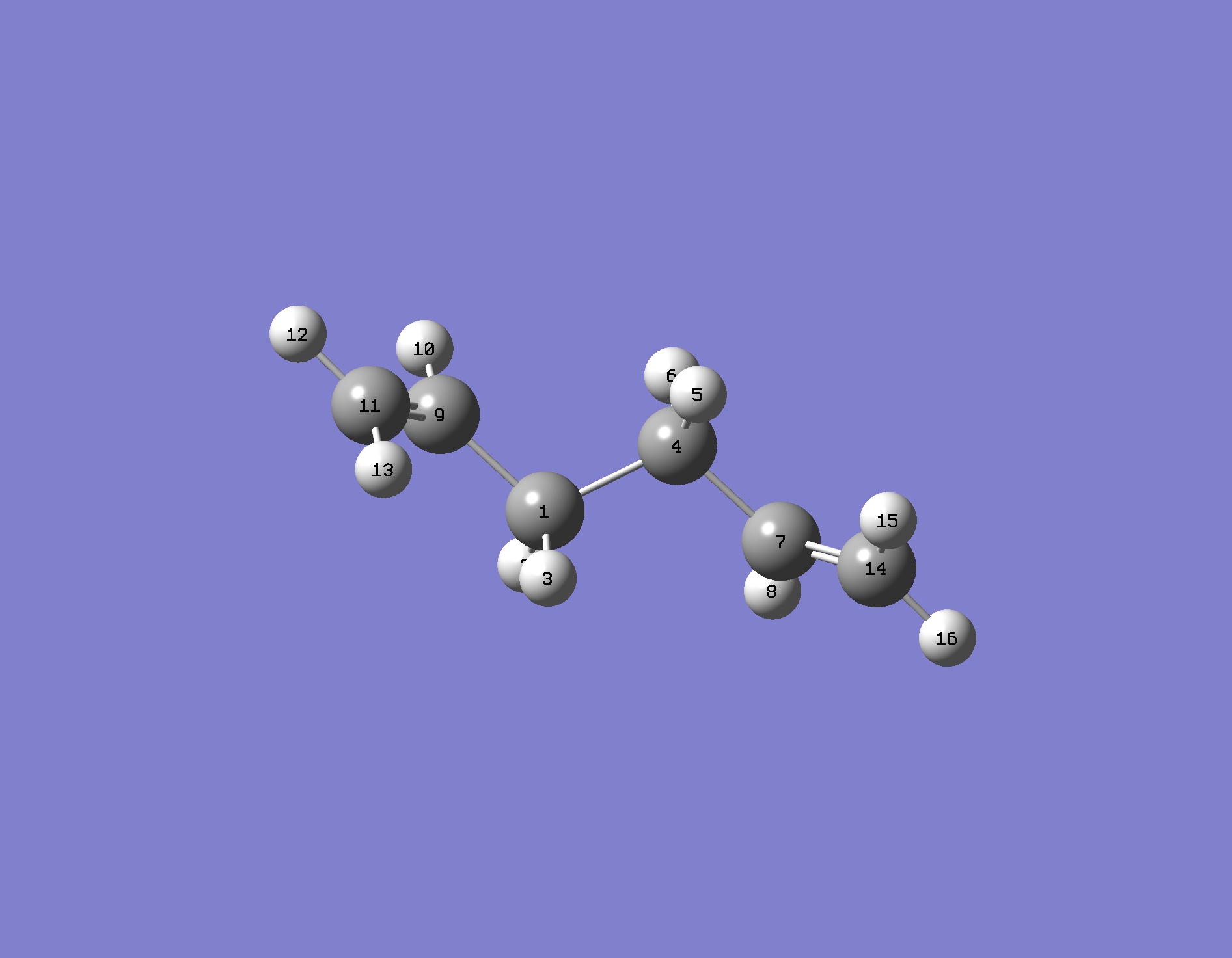
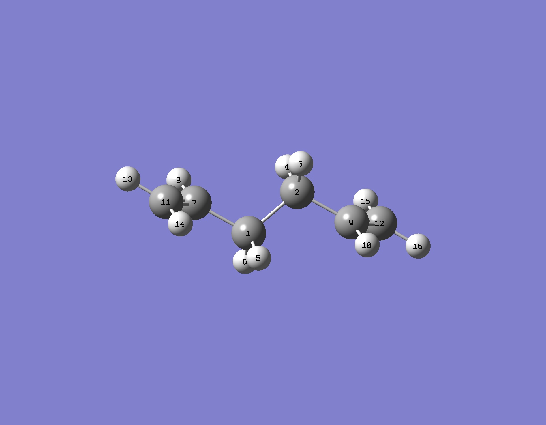
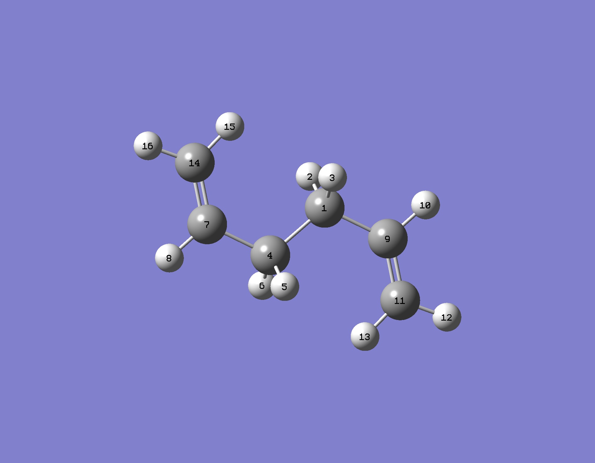
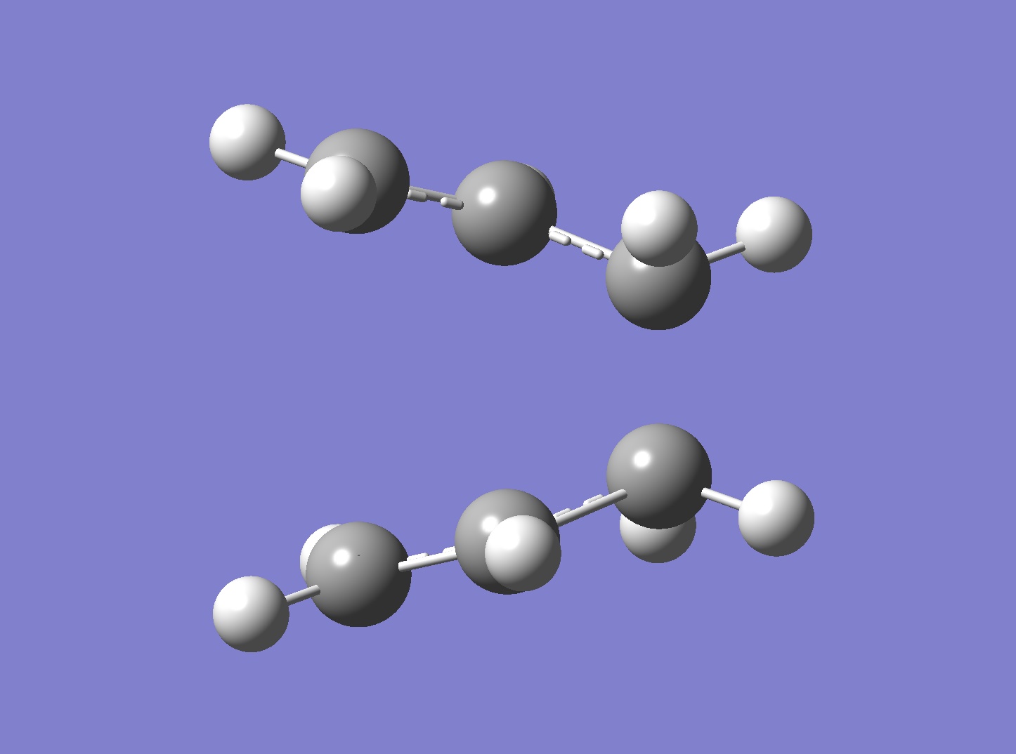
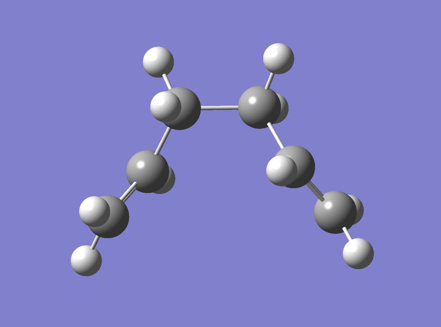
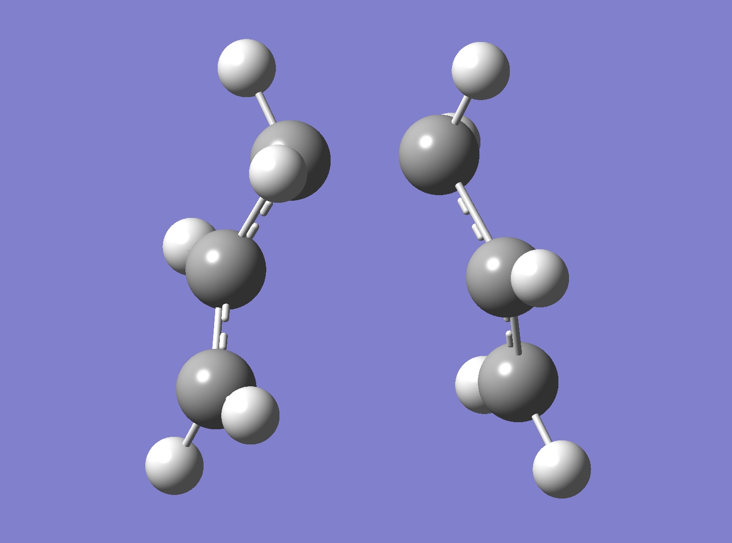
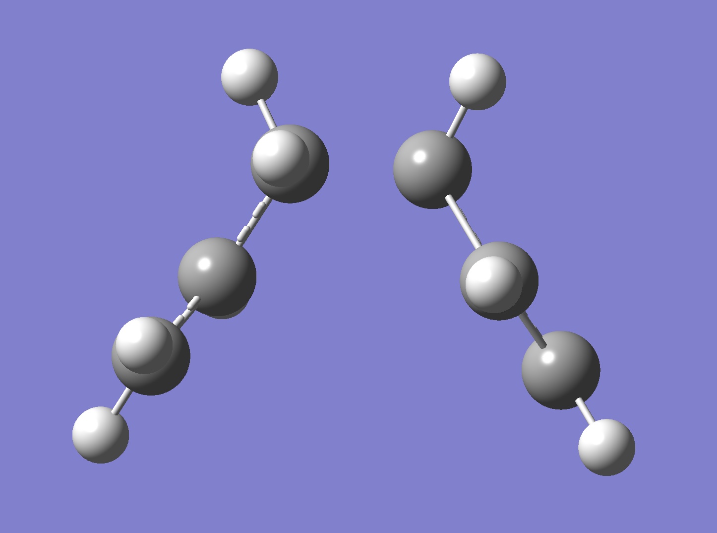
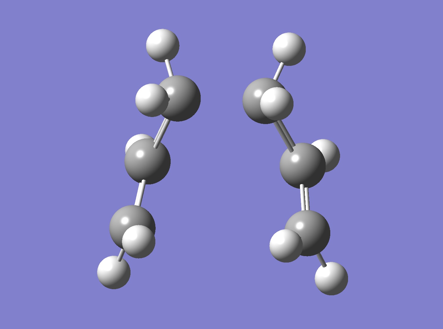
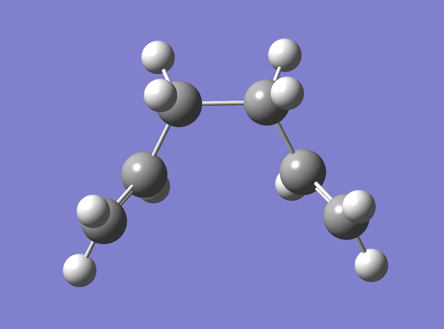
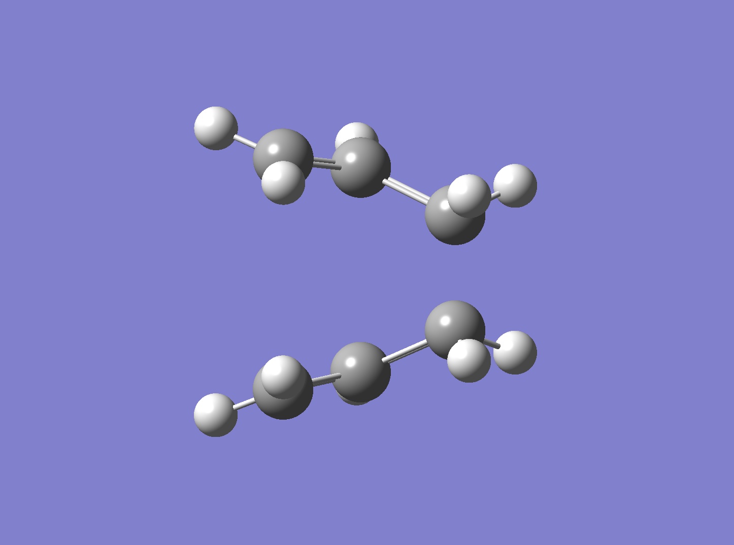
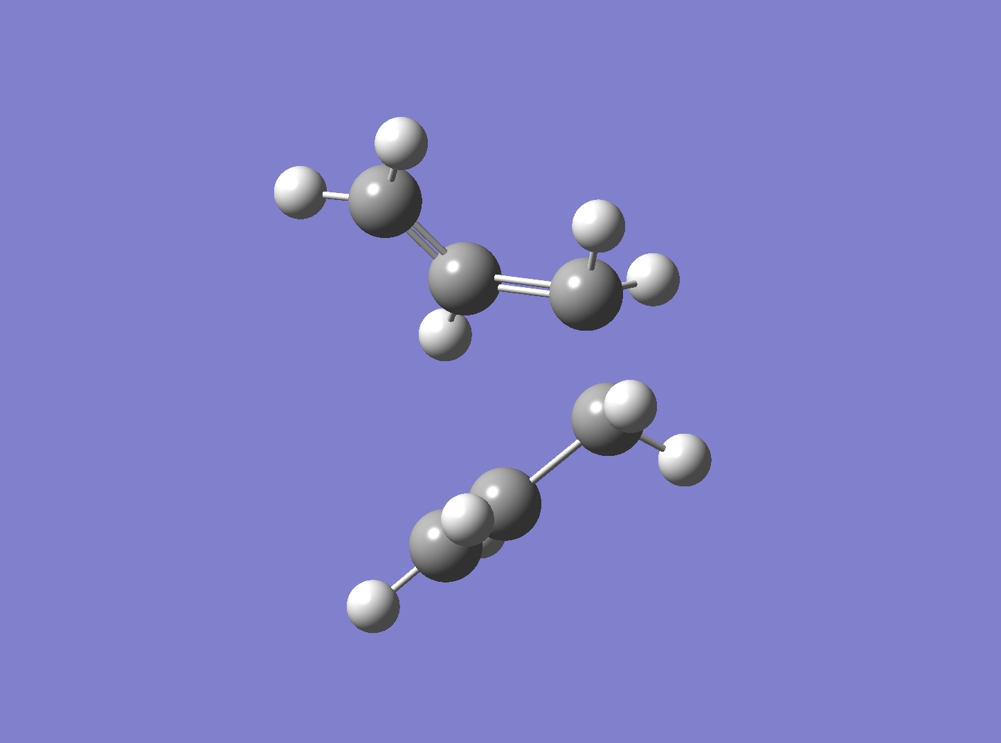
The low energy conformers (gauche and chair) of 1,5-hexadiene were optimized first using the HF/3-21G level of theory. The optimized energies and symmetry point groups were listed in Table 1. By inspection, the lowest energy conformer is the gauche 3 conformer. Due to the steric constrain, the gauche conformers are normally expected to be higher in energy than the anti conformers. This rather unexpected result here may be due to the presence of secondary orbital overlaps. Therefore the MO analysis was considered for gauche 3 in particular. As shown in Figure 2, it can be seen that some degree of secondary orbital overlaps in HOMO and LUMO exist for the gauche 3 conformer, particularly the HOMO has significant bonding πC=C orbital and anti-bonding π*C=C orbital overlaps, which is only true for the gauche conformation. Therefore it can be concluded that at the HF/3-21G level of theory, this effect is the dominant effect and renders the gauche 3 conformation the lowest energy.

Figure 2.MO Orbitals of gauche 3 conformer(HF/3-21G)

LUMO	HOMO

Table 1:Relative Energies of Conformers (HF/3-21G)

Conformer(Jmol)	Structure	log File	Energy/Hartrees HF/3-21G	Relative Energy/kcalmol-1	Point Group
gauche 1	Link to Structure	DOI:10042/to-13403	-231.68772	3.08	C2
gauche 2	Link to Structure	DOI:10042/to-13404	-231.69167	0.62	C2
gauche 3	Link to Structure	DOI:10042/to-13405	-231.69266	0.00	C1
gauche 4	Link to Structure	DOI:10042/to-13406	-231.69153	0.71	C2
gauche 5	Link to Structure	DOI:10042/to-13407	-231.68962	1.90	C1
gauche 6	Link to Structure	DOI:10042/to-13408	-231.68916	2.20	C1
anti 1	Link to Structure	DOI:10042/to-13415	-231.69260	0.04	C2
anti 2	Link to Structure	DOI:10042/to-13416	-231.69253	0.08	Ci
anti 3	Link to Structure	DOI:10042/to-13417	-231.68907	2.25	C2h
anti 4	Link to Structure	DOI:10042/to-13418	-231.69097	1.06	C1

By comparing the energies of different conformers, the relative energies ( to the lowest energy “gauche 3” conformer) were calculated and converted into kcal mol^-1 as shown in table 1. It can be seen that, the gauche 3, anti 1 and anti 2 conformers are closer in energies than other conformers (within 0.1 kcal mol^-1 range). This small amount of variations may be caused by systematic errors or instrumental errors. In order to investigate the lowest energy conformer, it is worth to calculate these conformers again but with higher level of theory. In here, the B3LYP/6-31G(d) level of theory was used. The anti 4 conformer (roughly 1 kcal mol^-1 differ to the gauche 3 conformer) was also optimized using the B3LYP/6-31G(d). This gives an idea of the difference in energy between the relatively high energetic conformers with the three of the lowest energetic conformers in the B3LYP theory.

Table 2:Relative Energies of Conformers (B3LYP/6-31G*) .

Conformer(Jmol)	Structure	Newman Projection	log File	Energy/Hartrees HF/3-21G	Relative Energy/kcalmol-1	Point Group
gauche 3			DOI:10042/to-13445	-234.61133	0.29	C1
anti 1			DOI:10042/to-13436	-234.61179	0.00	C2
anti 2			DOI:10042/to-13437	-234.61171	0.05	Ci
anti 4			DOI:10042/to-13438	-234.61079	0.63	C1

As shown in table 2, according to the B3LYP/6-31G(d) method, it can be seen that the anti 1 conformer has the lowest energy and anti 2 conformer has a energy within 0.05 kcal mol^-1 higher than that of anti 1 conformer. Although gauche 3 conformer is still low in energy, comparing the lowest energy, this differs by 0.29 kcal mol^-1. One can conclude that to explain the low lying energies of anti conformers is because the bonding σ_C-H orbital and the anti-bonding σ*_C-H orbital ovelap. This is also true for the bonding σ_C-C orbital and the anti-bonding σ*_C-C orbital. Infact, there are three competing effects here, all of them contribute to the relative energies of different conformers.

• Stablising Effect: bonding σ_C-H orbital/antibonding σ*_C-H orbital and bonding σ_C-C orbital/anti-bonding σ*_C-C orbital overlaps (Secondary Orbital Overlap): The effect is stablising the bonding orbital and destablising the anti-bonding orbital. Since the anti-bonding orbitals are always unoccupied, the overall effect is stablising the molecule. Both the gauche and the anti conformers have this effect, however anti-peri-planar(app) truns out to be stablised (optimal alignment) more than the gauche conformers.
• Destabling Effect: bonding σ_C-H orbital/bonding σ_C-H and bonding σ_C-C orbital/bonding σ_C-C orbital experiencing electron repulsion (Pauli repulsion): When two occupied molecular orbitals close to each other, this effect arises. This effect is particular larger between C-C bonds. Therefore the further away the C-C bonds, less pauli repulsion. Therefore the anti conformers experienece minimal electron repulsion effect.
• Stablising Effect: Van Der Waals (dispersion) interactions: This arises from the non-directly bonded atoms (typical H...H interaction ~ 2.2Å). By inspection, gauche conformer has two sets of H...H dispersion interactions, while anti conformers do not have this type of interactions. Therefore this effct only favours the gauche conformation.

Geometry Analysis

To compare the difference in geometry of the two different levels of theory, the bond distance/Å (C1-C2, C2-C3, C2-C3, C4-C5, C5-C6), bond angle/^o (C1-C2-C3, C2-C3-C4, C3-C4-C5 and C4-C5-C6) and torsional angles/^o (C1-C2-C3-C4 and C3-C4-C5-C6) are listed in Table 3. From both of the conformers, it can be seen that the two levels of theory roughly produce the same geometry. It seems that the C=C bond distances are slightly shorter for B3LYP method, while bond angles are larger compared to the HF/3-21G method. This is a good indication where small level of theory (HF/3-21G) is particular successful in predicting the structure of the molecules, while the electronic energy calculations are best obtained with large level of theory(B3LYP/6-31G*).

Table 3.Geometry Analysis of anti 1 and guche 3 conformers (comparing between HF/3-21G and B3LYP/6-31G(d))

Conformer (theory)	C1-C2 bond distance/Å	C2-C3 bond distance/Å	C3-C4 bond distance/Å	C4-C5 bond distance/Å	C5-C6 bond distance/Å	C1-C2-C3 bond angle/o	C2-C3-C4 bond angle/o	C3-C4-C5 bond angle/o	C4-C5-C6 bond angle/o	C1-C2-C3-C4 torsional angles/o	C3-C4-C5-C6 torsional angles/o
anti 1	1.32	1.51	1.55	1.51	1.32	124.8	111.4	111.4	124.8	-115.1	-115.1
anti 1	1.33	1.50	1.55	1.50	1.33	125.3	112.7	112.7	125.3	-119.1	-119.1
gauche 3	1.32	1.51	1.55	1.51	1.32	125.0	111.9	111.9	124.5	117.2	-120.9
gauche 3	1.33	1.50	1.55	1.50	1.33	125.5	113.5	113.5	125.5	119.4	-122.1

Frequency Analysis

Figure 2: gauche 3 IR Spectrum

Figure 3: anti 1 IR Spectrum

Figure 4: anti 2 IR Spectrum

Optimization of molecules is almost always the first step carried out in computational chemistry. Therefore it is important to ensure that the optimization performed goes to completion, otherwise further analysis (i.e. Molecular Orbital) cannot be valid. Gaussview allows to always checking whether the energy has been fully converged via looking at the first derivative of the energy (the first derivative equals to zero if the energy is at maximum or minimum in the reaction coordinate). Furthermore to determine whether it is a maximum or minimum, the frequency analysis is important. Frequency represents the second derivative of the electronic energy. Therefore positive frequency represents minimum energy is obtained, in other words, the optimization goes to completion. If the frequency is negative (imaginary frequency), this means that the maximum energy is obtained. In later Diels-Alder reaction, the negative frequency represents the maximum of the energy, which is effectively the same as the transition state.

Table 3: Frequency analysis of Conformers (B3LYP/6-31G*) .

Conformer(Jmol)	Sym. C=C str. Freq./cm-1 (Int.)	Sym. C=C str. Description	Asym. C=C str. Freq./cm-1 (Int.)	Sym. C=C str. Description	log File
gauche 3	1732 (7)	1732 (7)	1733 (6)	1733 (6)
anti 1	1732 (5)	1732 (5)	1735 (14)	1735 (14)
anti 2	1731 (0)	1731 (0)	1734 (18)	1734 (18)

As shown in figure 2, 3, 4, the absence of the negative frequencies in the IR spectra of all three conformers confirm that the optimization went to completion and the electronic energy is thus the minimum. Also the IR spectra confirm the structure of the conformers. For example looking at the C=C stretches, the anti 2 conformer is expected to have no symmetrical C=C stretches as the change in dipole moment is expected to be zero and thus IR inactive. The computated frequencies listed in table 3 agree to expectation, which indicates that the computational analysis is effective to predict the structure of the molecules.

Summary of Energies

The electronic and zero energies, the sum of the electronic and thermal energies, the sum of electronic and thermal enthalpies and the sum of electronic and thermal free energies of anti 2 conformer were obtained in the output file of the frequency analysis. These energies are listed in table xxx below. Representation of each energy term:

• The electronic and zero energy: the potential energy at 0 K, E = E_elec + E₀ (E₀ is the zero point energy)
• The sum of the electronic and thermal energy: the potential energy at 298.15K and 1 atm, E' = E + E_vibrational + E_rotational + E_{translational}
• The sum of the electronic and thermal enthalpy: energy correction contributions from RT is considered, H = E + RT
• The sum of the electronic and thermal free energy: Gibbs free energy, G = H - TS

To further investigate the relationships between these energies and the temperature and pressure, the nature of the partition functions can be obtained.

Temperature and Pressure Dependance

As instructions shown in the advanced Gaussian Tutorial, the Freq=Readisotopes option was used in order to obtain the temperature and pressure denpendance of the anti 2 conformer.

Temperature Dependance at 1atm Pressure

0K:DOI:10042/to-13657

100K:DOI:10042/to-13658

200K:DOI:10042/to-13659

300K:DOI:10042/to-13660

400K:DOI:10042/to-13661

500K:DOI:10042/to-13662

Conclusion:

• The sum of the electronic and zero-point energy does no vary with temperature, since they are essentially the same property calculated by partition fucntion.
• The sum of electronic and thermal energy and the sum of electronic and thermal enthalpy terms both increase as temperature increases, however by inspection, the electronic and thermal enthalpy term increase faster than the electronic and thermal energy term. This is because the extra RT term in the thermal enthalpy is also temperature dependant, this increases the gradient of the curve.
• The sum of electronic and thermal free energy term decreases as temperature increases, as G = H - TS, and H increases as temperature increases, therefore -TS is said to be decrease as temperature increases and this decrease is dominant effect in Gibbs energy calculation.

Pressure Dependances at 300K

0atm:DOI:10042/to-13660

5atm:DOI:10042/to-13663

10atm:DOI:10042/to-13664

20atm:DOI:10042/to-13665

50atm:DOI:10042/to-13666

100atm:DOI:10042/to-13667

Conclusion:

• The sum of the electronic and zero-point energy and the sum of electronic and thermal energy and the sum of electronic and thermal enthalpy terms do no vary with pressure , since they are essentially pressure independent.
• The sum of electronic and thermal free energy term decreases as pressure increases, as G = H - TS, and H remains the same as pressure increases, therefore -TS is said to be increase as pressure increases.

Transition State

Transition states are more difficult to optimize than the reactant/product optimization. While the optimization of reactant/product can be performed from large bond distance until the minimization occurs. However the transition state is already high in energy. To optimize the transition structure, a specific direction of the negative curvature in the reaction coordinate is needed before optimization, otherwise the optimization will end up with the structure of reactant/product.

Chair TS

The Force Constant Matrix (Hessian)

Since the transition state can be reasonbly well guessed for this simple reaction, the geometry can be optimized by computing the force constant matrix initallly. Then the force constant can be updated as the optimization proceeds.

Key word:

# opt=(calcfc,ts,noeigen) freq hf/3-21g geom=connectivity

As shown in the key word, the optimization was performed as to optimization to a TS(Berny), the force constant was calcuated once and the opt=noeigen was added in the additional keyword to prevent the gaussian from crashing (when more than one imaginary frequency is obtained).

Table 5: Properties of Chair TS (HF/3-21G)

Conformer(Jmol)	Electronic Energy/ Ha	Imaginary Freq./cm-1	Animation	log File
Chair TS	-231.61932	-818	Click to view animation

The Frozen Reaction Coordinate

This is an approach of optimizing the transition state if the structure cannot be guessed easily and correctly. The reaction coordinate (partly bonded C-C distance) was frozen first and then the frozen structure was optimized to reach the minimum energy. After optimizing the frozen molecules, the reaction coordinate was unfrozen. This molecule is then said to be fully relaxed. This method is particular powerful as by optimizing the frozen coordiante, the force constant generated is accurate compared to the real geometry. Therefore this can be drawn analogy to the force constant matrix method, instead of providing the force constant manually, the optimization of the frozen coordinate provides a good enough force constant to start with. This type of calculation saves relatively fair amount of computing resources.

Key words: initial frozen coordiante and optimization:

# opt=modredundant hf/3-21g geom=connectivity

relaxed coordiante and further optimization:

# opt=(ts,modredundant) freq hf/3-21g geom=connectivity

Table 6: Properties of Chair TS (HF/3-21G)

Conformer(Jmol)	Electronic Energy/ Ha	Imaginary Freq./cm-1	Animation	log File
Chair TS	-231.61932	-818	Click to view animation

Although the force constant matrix and the frozen coordinate methods are sufficiently to generate the optimized transition, however it is impossible to predict the reaction pathways from the transition states to products. The Intrinsic Reaction Coordinate method functioned in gaussian is a method to predict the reaction path. This allows the minimum path from the transition state to the product (not necessarily the product, as gaussian is only capable in finding the local minimum on the PES) to be followed step by step.

Intrinsic Reaction Coordinate

Initial Method: In this method, it can be seen that the intermediate geometries are not fully optimzed to the minimum geometry (Talbe 7). Therefore the reaction coordinate is need to be extended (to shorter bond distances).

# irc=(forward,maxpoints=50,calcfc) rhf/3-21g geom=connectivity

Table 7: Properties of Chair TS (HF/3-21G)

Conformer	Electronic Energy/ Ha (bond length/ Å)	log File	Animation	IRC Path
Chair TS(Click to View Final intrinsic structure)	-231.68604 (1.56)		Click to view animation

Intrinsic i: As shown in table 8, the first derivate of the energy is rougly approaching zero, which is a good indication of either minimum or maximum energy. Since the energy path is decreasing, it can be concluded that this is the local minimum energy. This is the fastest method to obtain the local minimum. However the correctness of the solution depend on the structure obtained from the initial IRC (final iteration).

# opt rhf/3-21g geom=connectivity

Table 8: Properties of Chair TS (HF/3-21G)

Conformer	Electronic Energy/ Ha (bond length/ Å)	log File	Animation	Optimization Path
Chair TS(Click to View Final intrinsic structure)	-231.69167 (1.55)		Click to view animation

Intrinsic ii: As seen from table 9, the structure is still the same same as the initial IRC method even though 500 points were optimized. Although this method is normally more reliable than the IRC i method, in here, its result is less good comprared to the IRC i method. This is because the IRC path is the wrong direction after too many points are calculated.

# irc=(forward,maxpoints=500,calcfc) rhf/3-21g geom=connectivity

Table 9: Properties of Chair TS (HF/3-21G)

Conformer	Electronic Energy/ Ha (bond length/ Å)	log File	Animation	Optimization Path
Chair TS(Click to View Final intrinsic structure)	-231.68604 (1.56)		Click to view animation

Intrinsic iii: This is the most realiable method. However as expected, to calculating the force constant always need more computing resources to perform. The result here is corresponds to the gauche 2 confromer with C2 symmetry. It is also worth to mentioned that this value agree to the IRC i method, therefore in the chair TS IRC path calculation, the normal minimization is the best method to locate the minimum energy path and follow that path to find the product with the minimum expenses.

# irc=(forward,maxpoints=500,calcfc) rhf/3-21g geom=connectivity

Table 10: Properties of Chair TS (HF/3-21G)

Conformer	Electronic Energy/ Ha (bond length/ Å)	log File	Animation	Optimization Path
Chair TS(Click to View Final intrinsic structure)	-231.69167 (1.55)		Click to view animation

Boat TS

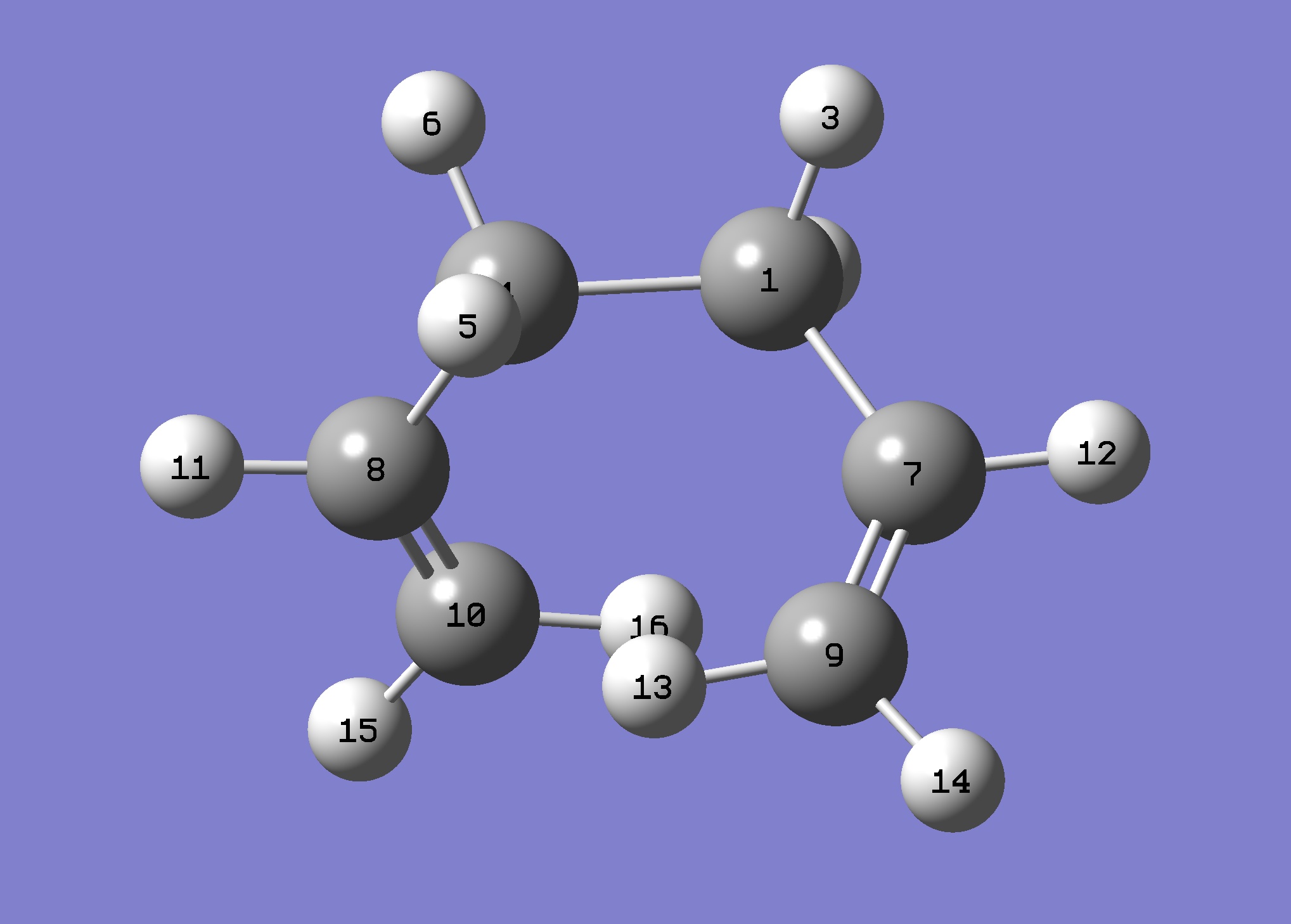
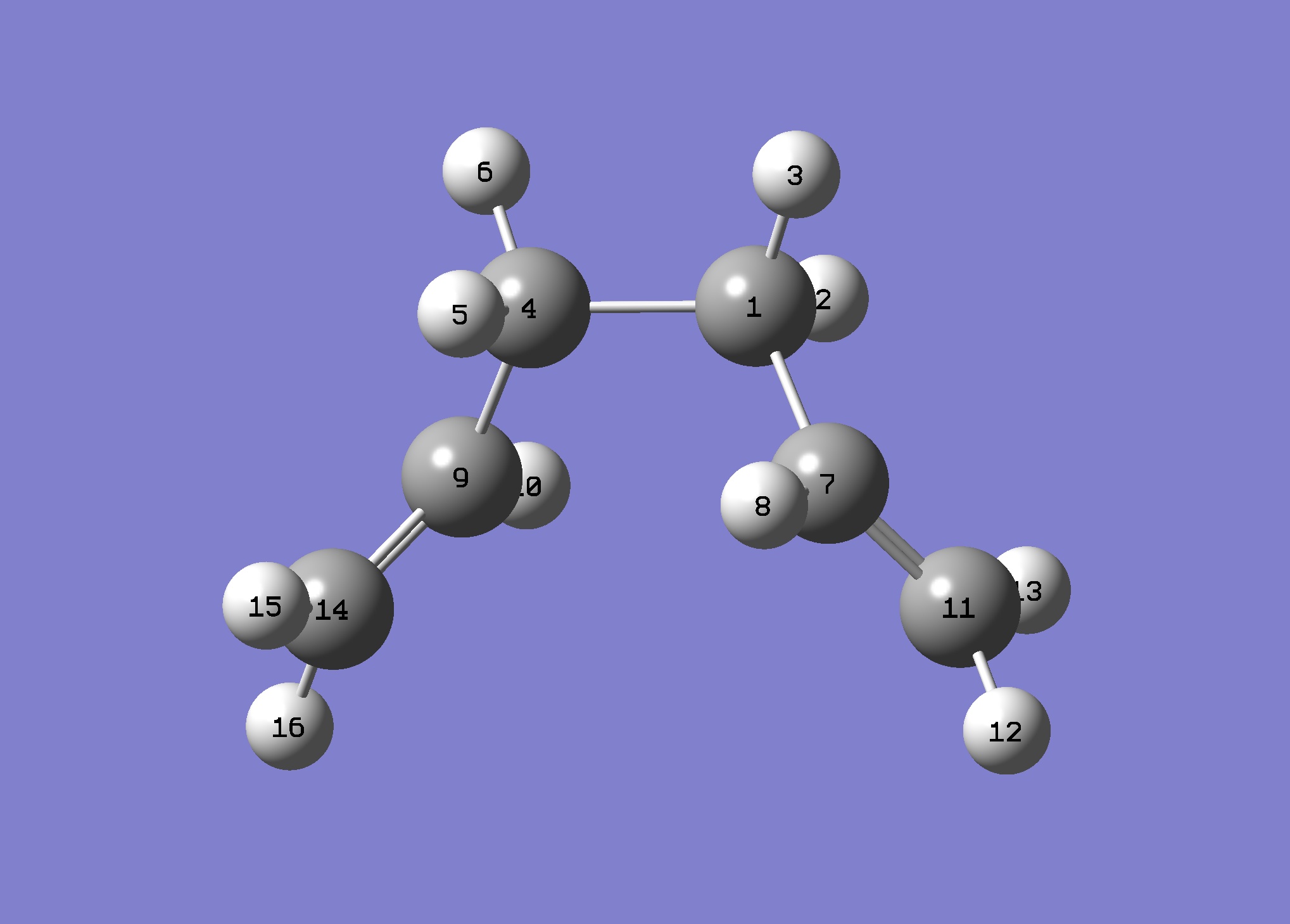
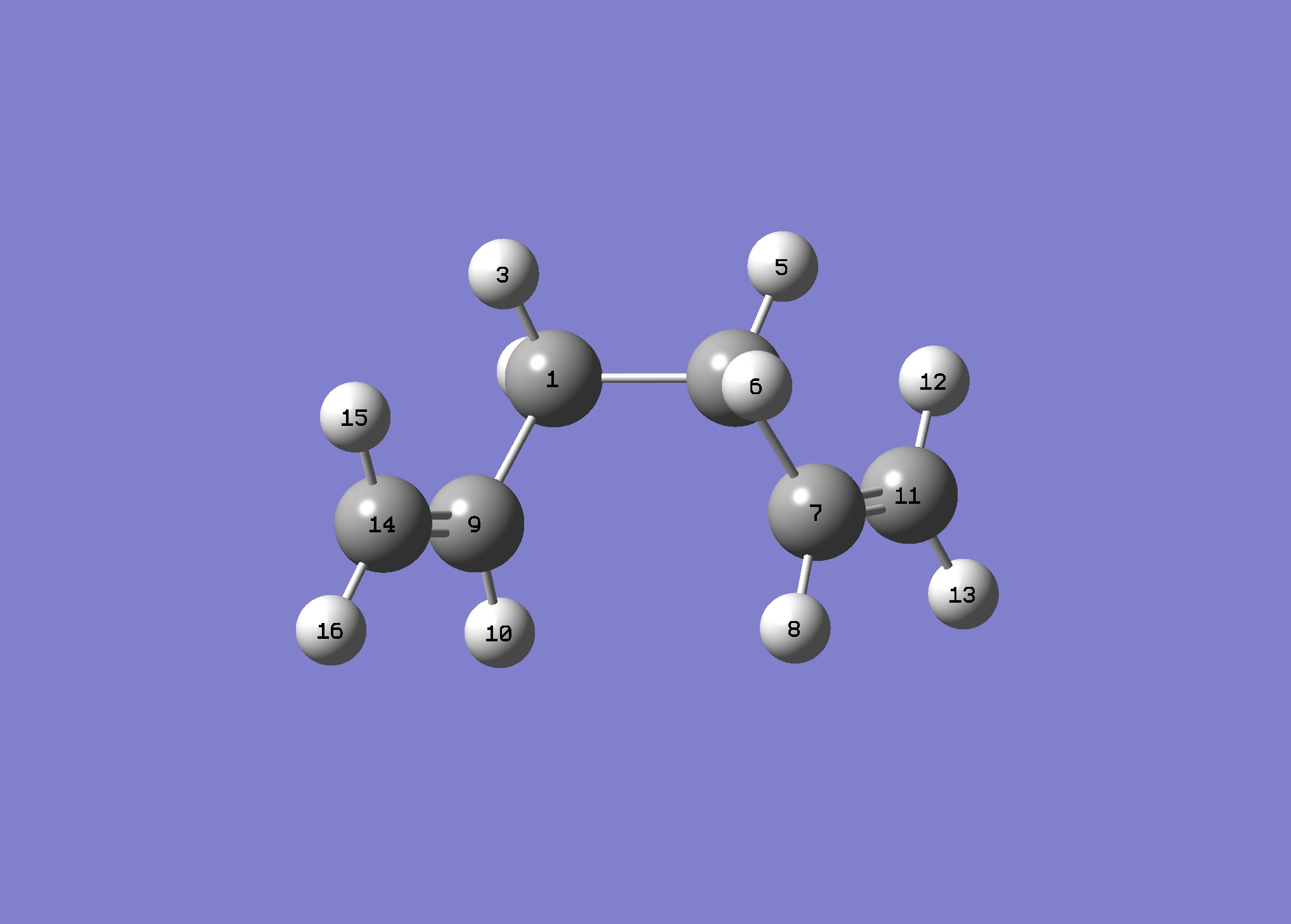
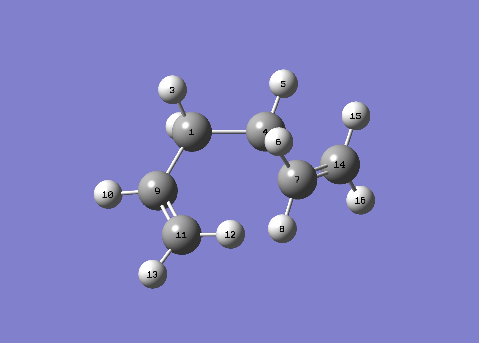
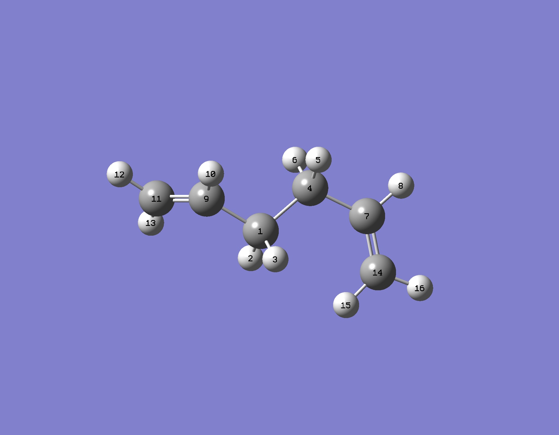
QST2 method The boat TS was optimized using another method called EST2. This method is very powerful if the transition state cannot be guesses properly. The reactants and products were specified with the same numbering system as shown in Figure 7. However the initial job failed as the QST2 method failed to rotate around the central bonds. Therefore the structure has to be rotated around and changed to a "more TS like" structure as shown in Figure 7 (C2-C3-C4-C5 dihedral angle is 0^o, C2-C3-C4 and C3-C4-C5 angle ~ 100^o). The energy obtained for boat TS is larger than that of chair TS, therefore the chair TS is the thermodynamically more favoured product.

# opt=qst2 freq hf/3-21g geom=connectivity

Figure 7 Input image of QST2 of boat TS

Table: Properties of Boat TS (HF/3-21G)

Conformer(Jmol)	Electronic Energy/ Ha	Imaginary Freq./cm-1	Animation	log File
Boat TS	-231.60280	-840	Click to view animation

Intrinsic Reaction Coordinate The intrinsic reaction coordinate method of the boat TS was carried out exactly as the chair TS.

Initial Method:

# irc=(forward,maxpoints=50,calcfc) rhf/3-21g geom=connectivity

Table 11: Properties of Boat TS (HF/3-21G)

Conformer	Electronic Energy/ Ha (bond length/ Å)	log File	Animation	IRC Path
Chair TS(Click to View Final intrinsic structure)	-231.67507 (1.59)		Click to view animation

Intrinsic i:

# opt rhf/3-21g geom=connectivity

Table 12: Properties of Boat TS (HF/3-21G)

Conformer	Electronic Energy/ Ha (bond length/ Å)	log File	Animation	Optimization Path
Chair TS(Click to View Final intrinsic structure)	-231.68303 (1.58)		Click to view animation

Intrinsic ii:

# irc=(forward,maxpoints=500,calcfc) rhf/3-21g geom=connectivity

Table 13: Properties of Boat TS (HF/3-21G)

Conformer	Electronic Energy/ Ha (bond length/ Å)	log File	Animation	Optimization Path
Chair TS(Click to View Final intrinsic structure)	-231.67507 (1.59)		Click to view animation

Intrinsic iii:

# irc=(forward,maxpoints=500,calcfc) rhf/3-21g geom=connectivity

Table 14: Properties of Boat TS (HF/3-21G)

Conformer	Electronic Energy/ Ha (bond length/ Å)	log File	Animation	Optimization Path
Chair TS(Click to View Final intrinsic structure)	-231.68303 (1.58)		Click to view animation

By comparing the obtained strucuture, the C1 point group indicates gauche 3 conformer is the product followed by this path.

Summary of TS

Table 15: Energy Summary of Cope Rearrangement

	HF/3-21G						B3LYP/6-31G*
	log File	Electr. energy	Sum of electr. and zero-point energies (0K)	Sum of electr. and thermal energies (298.15K)	Sum of electr. and thermal enthalpies	Sum of electr. and free thermal enthalpies	log File	Electr. energy	Sum of electr. and zero-point energies (0K)	Sum of electr. and thermal energies (298.15K)	Sum of electr. and thermal enthalpies	Sum of electr. and free thermal enthalpies
Reactant (anti2)		-231.69253	-231.53954	-231.53257	-231.53162	-231.57092		-234.61171	-234.46920	-234.46185	-234.46090	-234.50078
Chair TS		-231.61932	-231.46670	-231.46134	-231.46040	-231.49520		-234.55698	-234.41493	-234.40901	-234.40806	-234.44381
Boat TS		-231.60280	-231.45093	-231.44530	-231.44435	-231.47912		-234.54309	-234.40234	-234.39601	-231.39506	-231.43109

Table 16: Energy Summary of Cope Rearrangement/kcal mole^-1

	HF/3-21G		B3LYP/6-31G*		B3LYP/6-31G*
	Activation Energy (0K)	Activation Energy (298.15K)	Activation Energy (0K)	Activation Energy (298.15K)	Lit. Energy (0K)
Chair TS	-45.71	-44.70	-34.06	-33.16	-33.5±0.5
Boat TS	-55.60	-54.76	-41.96	-41.32	-44.7±2.0

Activation Energy: The activation energies in table 16 were obtained by subtracting the E and E' of either chair TS or boat TS with the corresponding E and E' of the anti 2 conformer. (E and E' are mentioned in the above discussions, please see Mod:xl3209module3#Summary_of_Energies)

Conclusion of Cope Rearrangement

• At HF level of theory, the relative energies of the possible reactant and product conformers are compared. The lowest conformer is the gauche 3 conformer. This is best explained by the π interactions. At B3LYP level of theory, the realtive energies of the possible reactant and product conformers are compared. This time, the lowest energetic conformer is the anti 1 conformer. This is best explained by the app alignment and σ orbital overlaps. (Detailed explaination: link to the optimization section aboveMod:xl3209module3#Optimization) It can be concluded that HF level is particular useful in optimising the correct symmetry of complicated systems, and further optimization using a higher level of theory (i.e. B3LYP). By doing so, the computing expenses can be greatly saved.
• TS optimization methods:

Force Constant Matrix method is very useful if the TS can be easily guessed with high degree of accuracy. The force constant is manually given. Frozen Coordinate method is used where TS cannot be easily guessed, and optimizing the frozen bond length, which provides a good force constant to carry out further optimization.QST2 method provides an approach from calculating TS from reactants and products. However this method is not sucessful unless the products and the reactants are oriented in similar TS like structure.

• IRC method enables the reaction path way to be calculated via many iterations. And following the routes, the products can be derived.

The Diels Alder Cycloaddition

Dienophiles (i.e. ethylene) and conjugated dienes (i.e. cis-butadiene) are normally undergo a [π4s + π2s] cycloaddition reaction to form a substituted cyclohexene system. This reaction is called Diels-Alder Reaction. The important application of Diels Alder reaction is to synthesis the cyclohexene ring system. The reaction mechanism is generally considered to proceed via single transition state (concerted reaction). The 2π orbital of the diene combine with the 1π orbital of the dienophile to formntwo new σC-C bonds. The Diels-Alder reactions are generally considered as heat initiated.

Ethylene & Butadiene Cycloaddition

Reactants

Three levels of theories (AM1, HF, B3LYP) were used in constructing the LUMO and HOMOs of the reactants (ethylene and cis-butadiene). These MOs can thus be used to discuss whether the Diels Alder reaction is allowed or forbidden.

Table 5: Cisbutadiene and Ethylene HOMO and LUMO

	Semi-empirial/AM1		HF/3-21G		B3LYP/6-31G*
log File	LUMO Orbital	HOMO Orbital	LUMO Orbital	HOMO Orbital	LUMO Orbital	HOMO Orbital
Cisbutadiene
Ethylene

By inspection,

• The MOs computated by three levels of theories are similar to each other.
• The interacting orbtials involve the 4π orbitals from the butadiene and the 2π orbitals from the ethene.
• The HOMO of ethylene is classified as symmetric (s) bonding MO, the LUMO of the ethylene is classfied as anti-symmetric (a) anti-bonding MO.
• The HOMO of butadiene is classified as anti-symmetric (a) bonding MO, the LUMO of the ethylene is classfied as symmetric (s) anti-bonding MO.
• Rules: HOMO-LUMO interaction allowed, HOMO-LUMO with different symmetries forbidden.
• Therefore the s HOMO of the ethylene can overlap with the s LUMO of the butadiene and the a LUMO of the ethylene can overlap with the a HOMO of the butadiene. These HOMO-LUMO pairs are close in energy, and thus energetically favoured to overlap.
• As a result, The HOMO should have two new σC-C bond formed with a symmetry.

Transition States

Table 18: Cisbutadiene & Ethylene Transition State

Methodlog File	LUMO Orbital	LUMO Orbital Symmetry	HOMO Orbital	HOMO Orbital Symmetry	Partly formed sigma C-C bond distance/A (angle/o)	Vib. Freq./cm-1 (lowest positive freq.)	Animation
Semi-empirial/AM1		s		a	2.12 (99.4)	-926 (192)
HF/3-21G		s		s	2.21 (100.3)	-805 (262)
B3LYP/6-31G*		s		s	2.27 (102.2)	-526 (195)

• Typical sp³ C-C bond length/Å = 1.53
• Typical sp² C-C bond length/Å = 1.48
• Typical VDW radius/Å =1.70
• The partly formed C-C bond distances calculated lie ~ 2.12-2.27Å, which is longer than the typical sp3/sp2 C-C bond length, but shorter than the 2 x typical VDW radius. This indicates that the partly formed C-C bond has part of a C-C single bond property and part of a VDW interaction. This corresponds to the nature of the transition state.
• As shown in table 18, the vibrational animation suggests that the formation of the two bonds are synchronous. The lowest vibrational frequencies are animations involving the bending of the C=C bond, this does not relate to the transition state as Diels Alder reaction are concerted.
• HOMO at the transition state should be a if considering the symmetry rule that one s ovelap with one a can only produce a symmetry. The AM1 theory does suggest this expectation. However going to higher level of theories, the HOMO of the TS becomes symmetric. There are several possible reasons for this: 1. HF and DFT theories involve more orbital mixings, this may change the symmetry. 2. It could be that the HF and DFT theories simply fail to deal with the molecular orbitals.
• The reason of why the reaction is allowed was explained above. The HOMO of the TS derived from the antisymmetric antibonding LUMO of the ethylene and the antisymmetric bonding HOMO of the butadiene. While the LUMO of the TS can be derived from the symmetric HOMO of the ethylene and the symmetric LUMO of the butadiene.

Naleic Anhydride & Cyclohexa-1,3-diene Cycloaddition

Introduction

Figure 9 Reaction Mechanism of Regioselective Diels Alder Reaction

Figure 10 Kinetic vs. Thermo. Control

Maleic anhydride and cyclohexa-1,3-diene undergo regioselective Diels Alder Reaction. As shown in Figure 9, the regioselectiviy of the reaction is considered to favour the endo adduct. Although the exo adduct is energetically more favourable, the kinetic effect renders the selectivity of the endo product. The kinetic effect can be best explain with illustrations as in Figure 10. The endo isomer is the major product due to its low energy barrier. In other words, the activation energy of the endo adduct adduct is lower than that of exo adduct. Therefore the endo transition state has lower energy than that of the exo transition.

Exo and Endo TS

Both exo and endo transition states were optimized via the frozen reaction coordinate method. Different levels of theories were used in order to draw comparisons between diffenct theories. The HOMO and LUMO of the exo and endo TS are listed in table 19 and table 20 respectively.

Table 19: Exo Transition State

Methodlog File	LUMO Side View	LUMO Top View	HOMO Side View	HOMO Top View	Partly formed sigma C-C bond distance/A (angle/o)	Vibrational Frequency/cm-1	Animation	Electronic Energy
Semi-empirial/AM1					2.17 (99.5)	-816		-0.05035
HF/3-21G					2.26 (96.3)	-648		-605.60359
B3LYP/6-31G*					2.29 (99.3)	-448		-612.67931

Table 20: Endo Transition State

Methodlog File	LUMO Side View	LUMO Top View	HOMO Side View	HOMO Top View	sigma C-C bond distance/A (angle/o)	Vibrational Frequency/cm-1	Animation	Electronic Energy
Semi-empirial/AM1					2.16 (99.8)	-811		-0.05137
HF/3-21G					2.23 (94.4)	-644		-605.61037
B3LYP/6-31G*					2.27 (97.8)	-447		-612.68340

• By comparing the electronic energies of the exo and endo transition states, it can be seen that the endo transition state has lower energies than those of the exo TS according to all three theories. This agree to the introduction earlieer.
• Again, the partly formed bond distances lie between 2.16 to 2.29 Å. This value is larger than the sp3/sp2 carbon carbon bond, but shorter than 2x the VDW radius. This truly describes the transition state is lying between the bonded structure and the non-bonded structure.
• The structural difference between the endo and exo TSs can be considered if the maleic anhydride fragment remains constant in the plane, rotating the cyclohexadiene around its centre of mass by 180 degree.

Steric Interaction and Secondary Orbital Effect

-"Secondary orbital overlap is a possible effect favouring the endo TS, while unfavourable steric interactions is a possible effect disfavouring the exo TS. In reality, it is very difficult to differentiate the orbital and steric effects, therefore the secondary orbital effect remained controversial"

• It can be considered that exo TS is more sterically hindered, as the constrain may exist between the briged-head group and the hetero ring system.
• Furthermore, the endo TS adapts the geometry such that the secondary orbital overlaps between the pi systems of the C=C and C=O bonds.
• By examining further MOs of the exo and the endo TSs, it is particular ture by looking at the HOMO-1 MOs, the secondary orbital overlap is distinctly exist in the endo conformer. While in the exo conformer, the angle and the distance between the secondary orbitals are impossible to overlap.

Table 21: Exo Transition State Fruther MOs

Method	LUMO+2	LUMO+1	HOMO-1
Semi-empirial/AM1
HF/3-21G
B3LYP/6-31G*

Table 22: Endo Transition State Further MOs

Method	LUMO+2	LUMO+1	HOMO-1
Semi-empirial/AM1
HF/3-21G
B3LYP/6-31G*

IRC paths

Table 23: IRC Reaction Path (B3LYP/6-31G)

Transition State	log File	Animation	IRC Path
Endo	DOI:10042/to-13769
Exo	DOI:10042/to-13768

Conclusion: In retro-diels Alder reactions, the kinetic vs thermodynamic control are important in determining the products. However when investigating the transition states, the steric strain and secondary orbital effects are taken into account. Computational methods, frozen coordinate and IRC paths are particular useful in investigating the structure of the transition state. Overall, computational analysis is proved to be an useful way to discover the TS of the Diels alder reactions