Rep:Liquid Simulations with milandeleev

The numerical answers for most of the tasks were correct. Explanations conveyed a adequate understanding for most "small" questions e.g. why atom positions were not initialised randomly. However, it is clear you do not really understand the scope of the LJ model and consequently that of your simulations (see comments). The report seemed rushed and not well thought out, and definitely not written in the style of a scientific paper trying to convey specific results/conclusions. .

Introductory Tasks

Velocity Verlet Algorithm

A completed spreadsheet containing a model of this algorithm for a simple harmonic oscillator may be found here. The position of local maximum error with respect to time can be modelled by the following equation:

$\max (E)=(5t-1)\cdot 8\times 10^{-5}$

In order to ensure that the total energy does not change by more than 1%, the timestep used must deceed 0.3 s. This lack of deviation is very important, as it ensures that the system obeys the law of conservation of energy, which means that it behaves in a physically consistent manner. In terms of the simple harmonic oscillator, then, it ensures that the observed wave frequency and period is constant due to the below equation:

$E=h\nu$

Atomic Forces and Derivatives

A single Lennard-Jones potential reaches zero when the internuclear separation $r_0=\sigma$. This can be calculated by following the below process:

$\varphi (r)=4ϵ(\frac{{\sigma }^{12}}{r_0^{12}}-\frac{{\sigma }^6}{r_0^6})=0$

$\frac{{\sigma }^{12}}{r_0^{12}}=\frac{{\sigma }^6}{r_0^6}$

$r_0^{12}{\sigma }^6=r_0^6{\sigma }^{12}$

$r_0=\sigma$

To calculate the force at this separation, it must be known that the force is the negative derivative of the energy with respect to the internuclear separation. Hence:

$F=-\frac{\mathrm{d}\varphi }{\mathrm{d}r}$

$-\frac{\mathrm{d}\varphi }{\mathrm{d}r}=\frac{24ϵ{\sigma }^6}{r^7}(\frac{2{\sigma }^6}{r^6}-1)$

Substituting in $r_0=\sigma$, then:

$F_0=\frac{24ϵ{\sigma }^6}{{\sigma }^7}(\frac{2{\sigma }^6}{{\sigma }^6}-1)$

$F_0=\frac{24ϵ}{\sigma }$

To calculate the equilibrium separation $r_{eq}$, the minimum point of the energy curve must be found. This can be achieved by differentiating the equation and equating it to zero, and solving for $r$, which is equivalent to finding the location whereat $F=0$.

$\frac{\mathrm{d}\varphi }{\mathrm{d}r}=\frac{24ϵ{\sigma }^6}{r_{eq}^7}(1-\frac{2{\sigma }^6}{r_{eq}^6})=0$

$\frac{2{\sigma }^6}{r_{eq}^6}=1$

$2{\sigma }^6=r_{eq}^6$

$r_{eq}=2^{\frac{1}{6}}\sigma$

The well depth $\varphi \left(r_{eq}\right)$ thereof:

$\varphi \left(r_{eq}\right)=4ϵ(\frac{{\sigma }^{12}}{r_{eq}^{12}}-\frac{{\sigma }^6}{r_{eq}^6})$

$\varphi \left(r_{eq}\right)=4ϵ(\frac{{\sigma }^{12}}{{\left(2^{\frac{1}{6}}\sigma \right)}^{12}}-\frac{{\sigma }^6}{{\left(2^{\frac{1}{6}}\sigma \right)}^6})$

$\varphi \left(r_{eq}\right)=4ϵ(\frac{1}{4}-\frac{1}{2})$

$\varphi \left(r_{eq}\right)=ϵ$

Should be negative epsilon for well depth. .

Atomic Forces and Integrals

The integral below is a generalised form to which boundary conditions can be applied.

$\underset{L_1}{\overset{L_2}{\int }}\varphi (r)=\underset{L_1}{\overset{L_2}{\int }}4ϵ(\frac{{\sigma }^{12}}{r^{12}}-\frac{{\sigma }^6}{r^6})\mathrm{d}r$

$\underset{L_1}{\overset{L_2}{\int }}\varphi (r)=4ϵ{\sigma }^{12}\underset{L_1}{\overset{L_2}{\int }}{r}^{-12}\mathrm{d}r-4ϵ{\sigma }^6\underset{L_1}{\overset{L_2}{\int }}{r}^{-6}\mathrm{d}r$

$\underset{L_1}{\overset{L_2}{\int }}\varphi (r)=4ϵ{\sigma }^6{[\frac{1}{5r^5}-\frac{{\sigma }^6}{11r^{11}}]}_{L_1}^{L_2}$

The limits $L_1=\{2\sigma ,2.5\sigma ,3\sigma \}$ and $L_2=\mathrm{\infty }$ can be applied as below. The final results apply for $\sigma =ϵ=1$.

$L_2=\mathrm{\infty }\therefore (\frac{1}{5(\mathrm{\infty }{)}^5}-\frac{{\sigma }^6}{11(\mathrm{\infty }{)}^{11}})=0$

$\underset{L_1}{\overset{\mathrm{\infty }}{\int }}\varphi (r)=4ϵ{\sigma }^6(\frac{{\sigma }^6}{11L_1^{11}}-\frac{1}{5L_1^5})=4ϵ{\sigma }^6\left(\frac{5{\sigma }^6-11L_1^6}{55L_1^{11}}\right)$

$\underset{2\sigma }{\overset{\mathrm{\infty }}{\int }}\varphi (r)=4ϵ{\sigma }^6\left(\frac{5{\sigma }^6-11(2\sigma {)}^6}{55(2\sigma {)}^{11}}\right)=-\frac{699\sigma ϵ}{28160}=-0.0248$

$\underset{2.5\sigma }{\overset{\mathrm{\infty }}{\int }}\varphi (r)=4ϵ{\sigma }^6\left(\frac{5{\sigma }^6-11(2.5\sigma {)}^6}{55(2.5\sigma {)}^{11}}\right)=-\frac{4391808\sigma ϵ}{537109375}=-0.00818$

$\underset{3\sigma }{\overset{\mathrm{\infty }}{\int }}\varphi (r)=4ϵ{\sigma }^6\left(\frac{3{\sigma }^6-11(2.5\sigma {)}^6}{55(3\sigma {)}^{11}}\right)=-\frac{32056\sigma ϵ}{9743085}=-0.00329$

Periodic Boundary Conditions

1 mL of water at STP has a mass of 1 g. Consequently, the number of moles of water in such a volume n and the number of molecules N is calculated below. The final result is N = 3.43 × 10²³ molecules.
.

$n=\frac{m}{M_r}=\frac{1}{18.01528}=0.0555084350618$

$N=n\cdot N_A=0.0555084350618\cdot 6.022140857\times 10^{23}\approxeq 3.343\times 10^{22}$

The calculation for the volume of 10000 molecules of water at STP is below. The final result is 2.99 × 10^-19 mL.

$n=\frac{N}{N_A}=\frac{10000}{6.022140857\times 10^{23}}=1.6605390404272\times 10^{-}20$

$V=m=n\cdot M_r=1.6605390404272\times 10^{-20}\cdot 18.01528\approxeq 2.992\times 10^{-19}$

If an atom at (0.5, 0.5, 0.5) in a unit cube with repetitive boundary conditions (like the game Snake) moves along a vector of (0.7, 0.6, 0.2), it will reappear in the cube at (0.2, 0.1, 0.7).

Reduced Units

For argon, the Lennard-Jones parameters are σ = 0.34 nm and ϵ = 120k_B.

$r=r^{*}\cdot \sigma =3.2\cdot 0.34=1.088\text{ nm}$

$ϵ=120k_B=1.656778224\times 10^{-21}J\approxeq -2.751\times 10^{-48}\text{ kJ/mol}$

This is way too small. Think about the order of magnitude you expect. .

$T=T^{*}\frac{ϵ}{k_B}=1.5\cdot 120=180\text{ K}$

Equilibration Tasks

Creating the Simulation Box

If atoms are generated with random coordinates, one atom could be generated in a position that overlaps with another atom. This would dramatically increase the overall energy due to intra-pair repulsive potentials, destabilising the system.

A relative lattice spacing of 1.07722 for a simple cubic lattice (1 lattice point per unit cell) generates a lattice point per unit volume density of 0.79999. Generating an atom at each lattice point for a 10×10×10 box produces 1000 atoms. A relative lattice spacing of 1.49380 for a face-centered cubic lattice (4 lattice points per unit cell) generates a lattice point per unit volume density of 1.2. Generating an atom at each lattice point for a 10×10×10 box produces 4000 atoms.

Setting the Properties of the Atoms

The following commands in LAMMPS have specific functions, as described below:

mass 1 1.0

This command creates a type 1 atom with mass 1.

pair_style lj/cut 3.0

This command instructs the program to compute Leonard-Jones pairwise potentials, using a cutoff point of 3.

pair_coeff * * 1.0 1.0

This command gives the force field coefficients (ϵ and σ) between two type 1 atoms.

As the initial positions and velocities have been specified, this is consistent with the Velocity-Verlet algorithm.

Running the Simulation

Using piece of code that references the input value means that the rest of the code need not be altered when the input is altered. Furthermore, other values that depend on the given timestep can also be linked straight back to the input value.

Checking Equilibration

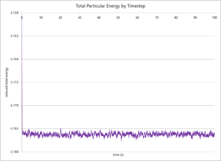
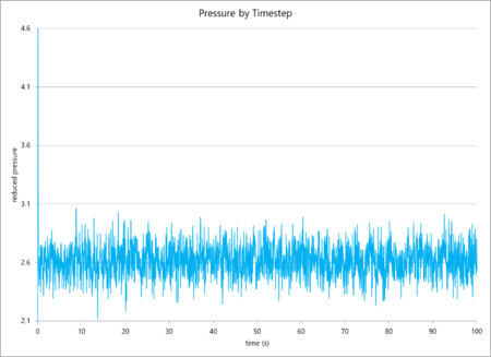
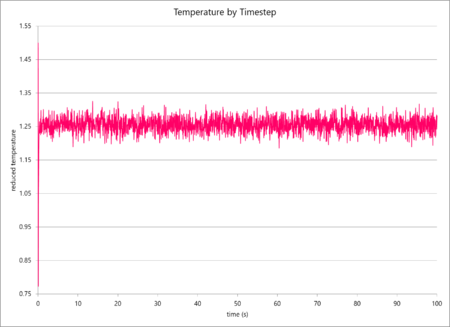
The simulation data of total particular energy, temperature and pressure against time for a 0.001 s timestep are graphed below (in that order). The simulation reaches a clear equilibrium for all three values, as, after a short period of time (ca. 0.03 s, or 30 timesteps).

Simulation Data

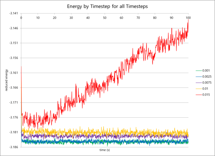
The data for different timesteps is graphed below. It is clear that the data for the 0.001 s and 0.0025 s are very similar and can essentially be used interchangeably. In the case of simulations over long periods of time, the 0.0025 s timestep is appropriate to reduce computation time but still maintain a high level of accuracy (the mean energy value differs by 0.005%). The 0.015 s timestep does not reach an average energy value, but instead continually increases the total particular energy with time: indicative of an unstable, positively feeding-back system. The Velocity-Verlet algorithm requires the initial atomic positions and velocities, and then simulates molecular movement from there. A large timestep results in large atomic displacements per timestep, causing a significant error in the calculation which multiplies by each timestep.

Comparison of Total Particular Energies for Different Timesteps

Specific Condition Simulations Tasks

Thermostats and Barostats

Setting γ as the velocity scaling factor to inter-convert between the instantaneous and target temperatures allows elucidation of its value in terms of the latter.

$\frac{1}{2}\sum _i{m}_i{v}_i^2=\frac{3}{2}N{k}_{B}T$

$\frac{1}{2}\sum _i{m}_i{\gamma }^2{v}_i^2=\frac{3}{2}N{k}_B\mathfrak{𝔗}$

$\frac{\frac{1}{2}\sum _i{m}_i{v}_i^2}{\frac{1}{2}\sum _i{m}_i{\gamma }^2{v}_i^2}=\frac{\frac{3}{2}N{k}_{B}T}{\frac{3}{2}N{k}_B\mathfrak{𝔗}}$

$\frac{1}{{\gamma }^2}=\frac{T}{\mathfrak{𝔗}}$

$\gamma =\pm \sqrt{\frac{\mathfrak{𝔗}}{T}}$

Examining the Input Script

In the program input scripts for the simulations in this section, there exists a line of code that resembles that below:

 fix aves all ave/time 100 1000 100000 v_dens v_temp v_press v_dens2 v_temp2 v_press2 

The first numerical variable (100 in this case) represents the number of timesteps τ_i over which an average is taken. Mathematically:

${\overline{v}}_n=\frac{\sum _i{\tau }_i}{100}$

The second numerical variable (1000 in this case) represents the number of averages over which to take a further average. Mathematically:

${\tilde{v}}_i=\frac{\sum _n{\overline{v}}_n}{1000}$

The third numerical variable (10000 in this case) represents the number of previous averages over which to take the final average. Mathematically:

${\hat{v}}_a=\frac{\sum _i{\tilde{v}}_i}{10000}$

Plotting the Equations of State

$\rho =\frac{p}{T}$

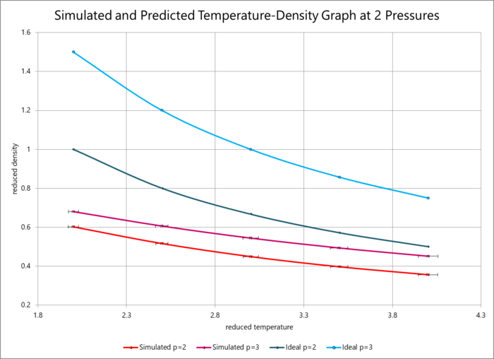
The data generated from the simulations in this section have been plotted in terms of temperature and density at reduced pressures 2 and 3 in the graph below (with error bars included). The ideal density calculated by the ideal gas law in reduced units (as above) is also plotted. The graph shows a clear discrepancy between the predicted and simulated densities, which is due to the ideal gas law treating the atoms as classical hard balls that experience no repulsion unless they are in direct contact (bouncing off each other). However, the Lennard-Jones potential models the atoms more faithfully to reality, in that, within a critical radius, the electrons orbiting the atoms repel each other and the atoms experience net repulsion. The densities predicted by the ideal gas are consequently higher as they do not take neighbour repulsions into consideration, which means that the model predicts that the atoms can be within closer proximities of one another without destabilising the system. You have to be careful to distinguish what your simulation "sees" (classical potentials) and what it is modelling (Pauli repulsion for the repulsive wall at close separations). It is not clear that you realise that classical models such as LJ coarse-grain out electronic degrees of freedom. .

However, it is also clear that the discrepancy decreases with increasing temperature. This is because, at higher temperatures, the atoms have more thermal energy and thus behave more like Newtonian hard balls, as their kinetic energy is dominant over the repulsive electronic forces until a smaller distance. Essentially, the atoms can get closer as their thermal energy can overcome the electronic repulsion.

Computed and Ideal Densities at varying Temperatures and Pressures

Statistical Physics Tasks

In this section, ten simulations were again run to determine the change in heat capacity per unit volume for a liquid at varying densities. An exemplar script can be found here. The results are graphed below. Higher density very obviously produces a higher heat capacity, which is expected because more atoms in one space can absorb more heat energy than fewer atoms in the same space. There is a clear decrease in the heat capacity with increasing temperature, which is at odds with the physical predictions. At lower temperatures, there are fewer thermally accessible translational, rotational, electronic and vibrational energy levels available. As temperature increases, more of these states become available so more of the energy levels become populated, making the internal energy rise rapidly. Since the heat capacity is the derivative of the internal energy with respect to temperature, higher temperatures are thus expected to increase the heat capacity (although this does level out towards the phase transition temperature). This deviation from the expected trend could possibly be explained by the fact that this system is modelling simple hydrogen atom fluids No it is not. ., and thus rotational and vibrational energy levels are not available. Furthermore the software itself may not take into account electronic transitions. Your simulation results look correct. However, one would expect that Cv is constant with T. .

Comparison of the Variation of Heat Capacities per Unit Volume with Temperature for Varying Densities

Radial Distribution Function Tasks

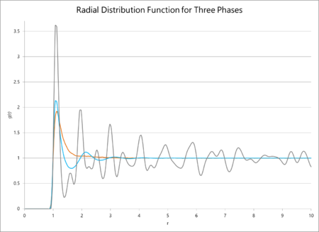
The radial distribution functions of multiple phases and their integrals are plotted against distance below. The radial distribution function for these simulations should average out to one, irrespective of the phase, because the function itself is a measure of the particle density surrounding a given particle. Consequently it can be seen as a measure of how consistently structured a material is: for a gas, the position of the particles is completely unpredictable and so it will very quickly tend to a central value. However, for a crystalline solid, the peaks will average unity but will never become a straight line that tend to unity, because the crystal has a defined structure with particles a fixed distance away from each other. Henceforth, there is a much greater probability that a particle will be found in a lattice site than outside of one, so the RDF will never lose its 'bumpiness'. From this line of reasoning, the RDF of a simple liquid should tend to unity but slower than the same function for a gas.

RDF and Integrated RDF for Three Phases

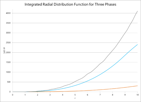To find the coordination number, the value of the first minimum on the RDF of the solid is found (which appears at $r=1.975$), which equates to a coordination number of 12. The lattice spacing, consequently, is ca. 1.37.

Dynamical Properties Tasks

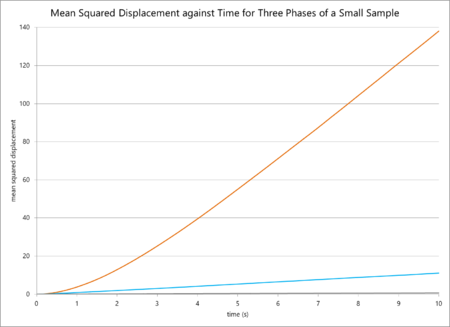
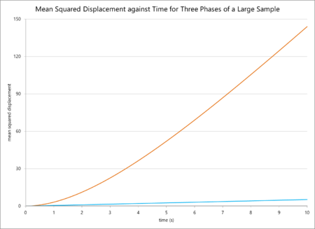
The mean squared displacements for a small sample and a large sample in different phases are plotted below.

Mean Squared Displacement for Varying Phases and Sample Sizes
Fewer Atoms	One Million Atoms

The resulting diffusion coefficients, calculated by the equation below (in which n is the dimensionality, or 3 in this case), are also tabulated below.

$\frac{\partial ⟨r^2\left(t\right)⟩}{\partial t}=2nD$

$D$ (m2s-1) to 8 s.f
Phase	Small Sample	Large Sample
Solid	0.010172398	5.4978008 × 10-7
Liquid	0.19168932	0.088731507
Gas	2.7676196	3.0690123

In general, these findings are logically consistent. The mean-squared displacement and thus the diffusion coefficient should be highest for a gas, as the particles have a higher thermal energy and so move away from their original positions fastest. Liquids have lower diffusion coefficients, and solids lower still. However, comparing the simulation for fewer and more atoms reveals some odd data. The diffusion coefficients for the gas phase are relatively similar, with a small increase on the side of the larger sample. This difference in value can simply be attributed to the greater accuracy of the million-atoms calculation. However, the value of $D$ for the liquid simulation is smaller for one million atoms, and for a solid it is much smaller still (by a magnitude of one hundred thousand). The values should at least be similar, as the parameters are similar, but the sample sizes are different. To rationalise this, it is possible to consider that the value for $D$ for one million atoms as a solid is skewed due to the presence of negative micro-gradient values, so it is difficult to compare in any valid sense to the computation for fewer atoms. For the case of the liquid, the origin of the difference is difficult to reason.

Academic Report

Abstract

Newtonian-esque simulations with Lennard-Jones pairwise potentials are used to simulate fluids and solids under different physical parameters, and the effects of varying these parameters are measured. The data is rationalised but more work is required to understand the effects of larger sample sizes. The abstract is meant to briefly summarise your results and conclusions, also briefly mentioning your methodology and motivations where applicable. After reading this abstract, I am still not sure what you have done: what physical parameters exactly? what is the "data" you have referred to? What were your results/conclusions? .

Introduction

Computational chemistry is an extremely broad area of research with wide-reaching implications for modern science. For systems more complex than a hydrogen atom, it is currently impossible to analytically solve the Schrödinger equation, which means that iterative and approximate solutions must be built. This is resource- and time-consuming work, and computation can make quick Only "quick" for small QM systems work of such laborious tasks Are you suggesting someone would attempt this by hand? . As computational simulations simulate real-life data what is "real-life data"? A very vague phrase. more and more accurately, this gives a way for programmers and scientists to more accurately fine-tune their algorithms I guess you are referring to benchmarking here - not very clear. Also you should benchmark computational models against experiment where available, and simulations where experimental data is lacking. , which bequeaths upon them, and, in turn, us, a better quantitative understanding of the quantum mechanisms Does it always? Most often we use QM to understand chemistry, not the other way around. that govern the behaviour of the microscopic. Conversely, this project in particular uses LAMMPS to model atomic behaviour, which utilises Newtonian approximations rather than purely quantum mechanical ones. This is because it requires far less computationally demanding simulations, and, in spite of the previous comments, this can also be useful: approximating real-life results without huge processing demand is a much easier and quicker alternative. In time, approaches such as these may be improved upon until their results may even match quantum mechanical methods to a large degree of accuracy, and it is to this advancement in classical modelling that this project aims to contribute Nowhere in this project have you improved upon classical-MD, parameterized more accurate force fields etc. .

The introduction is meant to provide the reader with the necessary background theory to understand what you have done in a paper, and also the motivation as to why what you have done is important. You have instead written a very vague and debatable overview of the field of computational chemistry..

Aims and Objectives

The aim of this exercise was to simulate particles of an ideal gas in different phases you have simulated different LJ phases, of which an ideal gas is the high T limit of the gas phase. , and compare their properties whilst varying different physical parameters, including particular density and temperature. It was important to the aims of this task that as much thermodynamic data could be extracted from such simulations as possible, as it is this data that can be verified physically. verified how? Using what data? To what physical system(s) do your LJ parameters correspond?

Methodology

Both the Verlet and velocity-Verlet algorithms were used in these simulations, with the initial positions and velocities set for the latter. All particles simulated were identical, and were used for 10000 timesteps. The simulations were run using LAMMPS, assuming particle interactions through Lennard-Jones pairwise potentials. The pairwise potential force field coefficients and particular masses were set to unity (in reduced units) and the cutoff point was between 3 and 3.2 units sigma. . Simulations were run for between 1000 and 10000 atoms with periodic boundary conditions enforced, in order to reduce simulation time This is not really why we use PBC. . The appropriate timestep was determined by equilibration, and a value between 0.002 and 0.0025 was determined to reduce computational time without sacrificing the accuracy offered by smaller timesteps. Why between x and y? You need to state exactly what you used, so it can be reproduced by another scientist. The same basic script input structure was utilised for each simulation, as below:

• the simulation box geometry was defined, including the lattice type (always simple cubic in this case), the number of repeat lattice units, the number density and the number of atoms
• the atomic physical properties were defined, including the mass, pairwise potentials, and Lennard-Jones cutoffs
• the thermodynamic state was established, including temperature and pressure or density
• the atomic velocities were established using the Maxwell-Boltzmann distribution and the simulation run to melt the crystal
• the thermodynamic parameters were re-imposed and the physical parameters measured, including temperature and density

Not necessary. You need just need to give the minimum amount of information for reproducability - not superfluous details about the input script.

When running simulations under specific conditions, the change in density according to temperature for this setup with a 15 × 15 × 15 lattice with number density 0.8 was recorded for temperatures of 2.0, 2.5, 3.0, 3.5 and 4.0 and pressures of 2.0 and 3.0. The true temperature, pressure and density along with standard errors were recorded and graphed.

When calculating heat capacities, the change in heat capacity per unit volume with temperature for a 15 × 15 × 15 lattice with number densities 0.2 and 0.8 was recorded for temperatures of 2.0, 2.2, 2.4, 2.6 and 2.8. The true temperature, density, volume and heat capacities were recorded, processed and graphed. The heat capacity was found using its relationship with the energetic variance:

$C_V=N^2\frac{\mathrm{Var}E}{k_B{T}^2}=N^2\frac{⟨E^2⟩-{⟨E⟩}^2}{k_B{T}^2}$

When calculating the radial distribution function for a 15 × 15 × 15 lattice in different phases, the number density and temperature for the solid, liquid and vapour phases were obtained from 'Phase Transitions of the Lennard-Jones System', Jean-Pierre Hansen and Loup Verlet, Phys. Rev. 184, 151 – Published 5 August 1969. Do not put full citation in-text. In these calculations, the gas density was 0.073 and temperature 1.5, the liquid density 0.606 and temperature 1.15, and the solid density 0.973 and temperature 0.75. The solid was assigned a face-centred cubic lattice structure. The trajectory files were then used in VMD to calculate the radial distribution function $g(r)$ and its integral, which were plotted for different phases against $r$.

When calculating the diffusion coefficient for a 20 × 20 × 20 lattice in different phases, the same density and temperature values from the previous calculations were used to calculate the total particular mean squared displacement, the derivative of which is equivalent to twice the product of the spatial dimensionality and the diffusion coefficient. In this case, the dimensionality is, naturally, three. The mean-square displacement was graphed as a function of time, and the pseudo-linear plots used to calculate a value for the diffusion coefficient. These plots were then compared with identical plots for one million atoms.

Results and Discussion

Computed and Ideal Densities at varying Temperatures and Pressures

The data from the simulations of specific temperatures and pressures (in blue colours on the graph) predicted that lower temperatures and lower pressures would produce a lower-density liquid, a logically consistent result. These results were also compared with predictions using the ideal gas law (in red colours), which produced densities much higher than expected: this is because the ideal gas law treats particles as classical Newtonian objects that repel simply through direct contact. The Lennard-Jones model is a more sophisticated way of treating particles that takes electronic repulsions beyond a critical radius LJ can be evaluated for all r not equal to 0. into account. The discrepancy between the simulated and calculated data, however, decreased with increasing temperature, as the large thermal energy of the atoms was able to overcome some of the electronic repulsion. and attraction. You have to be careful to distinguish what your simulation "sees" (classical potentials) and what it is modelling (Pauli repulsion for the repulsive wall at close separations).

Comparison of the Variation of Heat Capacities per Unit Volume with Temperature for Varying Densities

The data from the simulations of specific temperatures and densities predicted that the heat capacity of the liquid fell with temperature, and that it was higher with pressure. The latter result is logically consistent, as higher pressure (red on the graph) increases the internal energy of the fluid which means that more energetic states are available to populate, increasing the ability of the substance to absorb energy without heating up. Furthermore the energy states become closer together. However, the former result is very odd, as higher temperature, like higher pressure, should make higher-energy states more accessible and thus increase the specific heat of the fluid. However, this is not the case, and this could be attributed to the lack of vibrational, rotational (and possibly electronic) degrees of freedom for this particular system due to the atomic identities.

RDF and Integrated RDF for Three Phases

The data from the simulations of radial distribution functions and their integrals predicted a smooth tendency of the RDF towards unity for a gas, a slightly less smooth tendency for a liquid, and an outright fluctuation of the solid around an average value of unity. This makes sense in all cases: a crystalline solid should not see an equal probability of finding a particle anywhere because it has an ordered structure which means that, in certain points, there will almost never be an atom. However, a gas is much more entropic is the word "entropic" as an adjective scientifically meaningful? What are you trying to say? Use precise language. , so the probability of finding a particle anywhere evens out more rapidly. The coordination number of the solid can easily be found from the value of the integral of the RDF at the first minimum point of the graph.

Mean Squared Displacement for Varying Phases and Sample Sizes
80,000 Atoms	1,000,000 Atoms

$D$ (m2s-1) to 8 s.f
Phase	Small Sample	Large Sample
Solid	0.010172398	5.4978008 × 10-7
Liquid	0.19168932	0.088731507
Gas	2.7676196	3.0690123

The data from the simulations of mean squared displacement against time predicted a smooth, almost-linear increase in MSD (and, thus, the diffusion coefficient) with time, and a higher MSD for gases than liquids and liquids than solids. This absolutely corresponds with scientific reasoning: particles in more disordered states at higher temperatures will experience larger displacements from their original positions. The solid phase especially experiences very little diffusion due to the compact, tightly-bound nature of the particles. However, when comparing the simulations for 80,000 and 1,000,000 atoms, the values diverge. The values for a gas are similar but the values for a solid are significantly lower for more atoms. Looking at the graph reveals some sources: the diffusion coefficient was calculated from the mean of the gradient of the linear portion of the plot, but there are some negative derivative values on the solid line for 1m particles that could skew the data. Furthermore, there could have been a change in density, pressure or temperature parameters when the sample size was increased, all of which would greatly influence the value of the mean-squared displacement. Surely these are specified as input parameters, why are you unsure as to whether they are different?

Conclusion

This experiment was successful in simulating small numbers of atoms in varying phases under different thermodynamic parameters to extract physical data. It is now important to investigate the effect of greater sample size (number of atoms considered) on the accuracy of the data as there were significant deviations between the million and eighty-thousand atom calculations. Specific molecular interactions, such as hydrogen bonding, should also be taken into account, in order to better simulate real-life systems. You have simulated a LJ solid/liquid/gas, which does not correspond to any "real life" system unless paramaterized to do so. Why do you think name H-bonding as something to include? It would indeed be important for some specific systems, and not at all important for others. What if you were trying to model a nobel gas (for which LJ is an appropriate choice), why would you include "molecular" interactions for a monatomic system.