Rep:Ha3915liqsim

Overall feedback. There is evidence of a generally good overall understanding, with all the major points being communicated. Some of the technical aspects of the molecular dynamics simulations were not understood or communicated well. Writing, while fine, could have been more precise and better edited. For example Diffusion coefficient or Mean squared displacement were sometimes capitalised mid sentence. Please note that I have included some technical details in the feedback; you were not expected to know these, and are just for your information. Mark: 63/100.

Abstract

Molecular dynamics simulations were used to calculate physical, structural and dynamic properties of a system. The radial distribution function for a solid, liquid and vapour were plotted as well as their integrals. the Mean squared displacements were also calculated and plotted leading to the calculation of the diffusion coefficients for the aforementioned phases. These were determined to be 2.12 x 10^-7 m² / s , 0.0859 m² / s and 2.81 m² / s for solid, liquid and vapour respectively. Throughout the various simulations it was noted that the decrease in order when going from solid to vapour can lead to massive changes in thermodynamic properties such as heat capacity. Good abstracts tend to include 1-2 sentences of motivation. Try to be more concise: for example, it is enough to say "mean squared displacements and diffusion coefficients were calculated" instead of "...calculated and plotted leading to the calculation of diffusion coefficients for the aforementioned phases". You should also summarise your results: what were the "massive changes".

Introduction

Molecular dynamics simulations utilise classical Newtonian mechanics Yes and no: Lagrangian mechanics. This is a technical point. to predict the motion of particles in an ensemble I assume you mean for trajectory propagation. AIMD simulations use QM methods for force evaluation. You have performed classical MD. . The computational power of multiple CPU cores, or in some cases GPU cores using the program allows the calculation of motion of multiple particles and how they interact with each other Not relevant, and not strictly true. These calculations could be done on a single core. Whether you can perform a given simulation depends on it's cpu-hour cost not just the number of CPUs . This computational chemistry technique enables us to predict the physical and thermodynamic properties of systems such as total energy, heat capacity and density; which would otherwise be very expensive, difficult or in some cases, impossible to calculate with a physical experiment.

Recently molecular dynamics simulations have been exploited throughout chemistry and medicine with successful simulations leading to new discoveries relating to protein folding and cancer treatment. since the function of a protein relies on the structure and stereochemistry (for example, to be able to form enzyme-substrate complexes) many new treatments rely on being able to simulate the structure of proteins at various thermodynamic constrains which may occur in the body. For example, matrix metalloproteinases (MMPs) are a class of Zn²⁺ containing proteins which help to promote the spread and survival of a cancer tumour through angiogenesis (the formation of new blood vessels for cancer cells). Inhibitors of MMPs are therefore wanted such that angiogenesis is controlled and possibly even antiangiogenesis for treating cancers. Molecular dynamics simulations are required for evaluating the intermolecular interactions between zinc and its coordinates and for performing nanosecond length-scale molecular dynamics simulation of zinc proteins. Nice that you've used a reference, however your report is not a review on molecular dynamics. .

Aims and objectives

The Aim of the simulations was to determine the dynamical and thermodynamic properties of a simple liquid system as the physical properties were varied and comparing these properties with similar structures in different phases. The density of the system was explored as a function of temperature, as well as the change in the radial distribution function (RDF) and its integral and the diffusion coefficient of the system for the solid, liquid and gas phases using two different data sets.

Methods

The main program used to execute the simulations was the Large-scale Atomic/Molecular Massively Parallel Simulator. (LAMMPS) which is designed specifically, with parallel programming to exploit the use of multi-core processors. The other program, used to visualise the trajectories exported by LAMMPS was Visual Molecular Dynamics (VMD), which utilises the OpenGL graphics library as well as CUDA acceleration to display the simulated system of the simulated simulation. Only crediting LAMMPS is sufficient, especially since you have not included the mentioned trajectories. .

The Lennard-Jones (LJ) potential was the potential of choice in LAMMPS "in LAMMPS" makes this confusing. You're potential of choice was LJ,

LAMMPS does not need to be mentioned. and is defined as follows:

$\varphi \left(r\right)=4ϵ(\frac{{\sigma }^{12}}{r^{12}}-\frac{{\sigma }^6}{r^6})$

Where

$ϵ$

is the well-depth and

$\sigma$

is the inter-nuclear distance at zero potential. Both of these had a set value of 1.0 and a cutt-off value of 3.0 was used such that the computer didn't have to calculate the pair potential between particles greater than 3.0 apart in reduced units; otherwise the simulations would've been computationally intensive and possibly impractical Only if a ridiculous cutoff was used. LJ is really very cheap, and you were not using incredibly large system sizes.. Only one type of particle was used and had a mass of 1.0 - all particles were identical.

Firstly, an NVE ensemble was simulated. A cubic 15 x 15 x 15 unit cell lattice with density = 0.8 reduced units was melted under specific conditions such that a liquid phase, with short range order, is achieved. The particles were then assigned a random velocity such that the Maxwell-Boltzmann distribution of speed was satisfied for the simulation.

An NPT ensemble was then simulated to allow controlled variation of temperature and pressure. This allowed the exploration of the change in density with temperature (T* = 2, 2.2, 2.4, 2.6, 2.8 ), at different pressures (P* = 1.8, 2.6).

Furthermore an NVT ensemble was used to allow the calculation of the heat capacity of the system for the same temperatures as above but for different densities (ρ* = 0.2 , 0.8). The radial distribution function was also determined for the three phases of solid, liquid and vapour, with the following T*, ρ* combinations which were determined by looking at the phase diagram.

	Solid	Liquid	Vapour
T*	1.0	1.2	1.2
ρ*	1.2	0.8	0.08

The diffusion coefficients were also calculated using the total mean squared displacement of the particles (MSD) and the velocity auto-correlation function (VACF) of the system.

Results and Discussion

You've used very small text size (unreadable) for plot axes. Some of the feedback is below in tasks. .

Density vs. Temperature - an NPT ensemble

Figure 1: Plot of Density vs. Temperature from the simulation with error bars compared with the prediction of the ideal gas law at 2 different pressures

As shown in Figure 1, the general trend is that density decreases with temperature, and increases with pressure. This is because at higher temperatures, the particles have more kinetic energy to overcome to attractive forces between each other slightly, and therefore there are fewer particles per unit volume. As for the pressure, the greater the pressure, the more "squeezed" the particles are in the volume and hence density increases with pressure.

As expected, the Ideal gas prediction is always higher than the simulation, this is because the Ideal gas law assumes point particles with no interactions and only fully elastic collisions. This neglects the repulsive interaction as the particles get too close to each other - this is accounted for in the simulation by the LJ potential. This difference between the Ideal gas law is even more observable at higher pressures as more particles are being forced closer to each other and therefore more repulsive forces are being ignored.

It should also be noted that the instantaneous rate of change of density with temperature is much greater for the Ideal gas law prediction compared with the simulation. As such, the accuracy of the ideal gas prediction increases at higher temperatures. This is because the particles have greater kinetic energies and are therefore less likely to experience the repulsive force as much as they will be further away from each other.

Heat Capacity vs. Temperature - an NVT ensemble

Figure 2: plot of heat capacity (per unit volume) vs. temperature for two densities (0.2, 0.8)

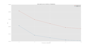
As shown in figure 2, the heat capacity of a system is higher at a higher density at all tested temperatures. This is because at higher densities, there are more particles/unit volume and as such more energy levels must be excited before an increase in temperature is seen thus, more energy is needed to excite the system to a higher energy state to raise the temperature of the system as per the definition of heat capacity.

The general trend is that heat capacity decreases with temperature as shown in figure 2. As the particles have more energy at higher temperatures, there is an increased density of states in the excited region thus the heat capacity decreases as it takes less energy to heat the system to higher temperatures due to the decreasing atomic energy gap sizes with further excitation.

The radial distribution function (RDF)

Figure 3: Plot of the radial distribution function for solid, liquid, vapour.

Figure 4: Plot of the integrated radial distribution function for solid, liquid, vapour.

As can be seen in figure 3, the RDF of the solid phase fluctuates fluctuates is not the right word: the peak structure arises from periodic order, and g(R) does not fluctuate wrt. r in the same way e.g. an timeseries of temperature or potential energy. much more than that of a liquid or vapour - it has significantly more maxima and minima. It also does not fully decay to 1 as with the other phases. This is due to the ordered nature of a solid lattice where the atoms positions are quasi-constant; as such the structure is periodic. Thus the number of maxima represents the different coordination shells that could surround the particle. The solid RDF does not decay to 1 (the bulk density) as the other phases because of the long range order of the solid structure.

The reduction in the number of maxima/minima in the liquid and vapour phases is largely due to the increased motion of the particles - losing long range order/structure. As expected the liquid phase has more peaks than the vapor phase due to the short range order found in liquids and therefore some coordination shells exist.

For the gas, the rapid decay suggests that there is very little order and the particles have very little locality, as such there are very few attractive potential forces Think more about what you have changed in the input file and how this translates to the PES and distribution of PE and KE. and hence the rapid decay. I understand what you are trying to convey. Try to be more precise with your choice of words. A particle's "locality" is a vague description.

Figure 4 shows the integrated RDF, which can be used to predict the coordination shells by comparing the running integral to the maxima in the RDF. In the solid RDF it can be seen that there are 3 coordination shells corresponding to the first 3 maxima which correspond to the initial coordination shells of an fcc lattice of 12, 6 and 24 atoms respectively.

Mean squared displacement (MSD)

Figure 5: Solid MSD from simulation of 1000 atoms.

Figure 6: Liquid MSD from simulation of 1000 atoms.

Figure 7: Vapour MSD from simulation of 1000 atoms.

Figure 8: Solid MSD from simulation of 1,000,000 atoms.

Figure 9: Liquid MSD from simulation of 1,000,000 atoms.

Figure 10: Vapour MSD from simulation of 1,000,000 atoms.

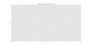
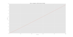
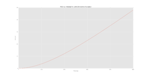
Figures 5-7 show the MSD calculations of the simulation whereas figures 8-10 show the plots from the data given for 1,000,000 atoms. Axes text is very small. I cannot read the scales. Could the data from some of these plots been plotted together? There are a lot of plots. .

The following diffusion coefficients were calculated from the MSD plots by using the following equation:

$D=\frac{1}{6}\frac{\partial ⟨r^2\left(t\right)⟩}{\partial t}$

The results are shown in the table below:

Diffusion coefficient table header with units included should have been used. .

Number of atoms	Solid	Liquid	Vapour
1000	2.12 x 10-7 m2 / s	0.0859 m2 / s	2.81 m2 / s
1,000,000	8.33 x 10-6 m2 / s	0.0871 m2 / s	3.08 m2 / s

The diffusion coefficient of the solid is very small, as expected, since there is very little motion (simply just vibrations) of the atoms in the lattice. This is supported further by the initial fluctuation of the MSD for the solid where the atoms are attempting to "escape" the lattice structure and thus the position of the atoms is approximately constant.

For the liquid and vapour phases, the particles are able to diffuse across, following brownian motion. The relationship between the MSD and time then becomes linear as the system moves from a ballistic regime to the diffusive regime.

It should be noted that the diffusion coefficient increases from solid to liquid to vapour which is what is expected as there is more free movement in a vapour than in a solid, the values for 1000 atoms are also similar in terms of orders of magnitude to the values with 1000000 atoms.

Conclusion

The molecular dynamics of solid, liquid and vapour systems were successfully simulated using LAMMPS with an LJ potential. The variation of thermodynamic properties with physical and structural properties was explored. For example the variation of density with temperature and pressure showed a decrease in density with an increase in temperature but an increase in density with pressure. A simple explanation is due to the kinetic energies of the particles increasing with temperature. Furthermore, the RDF and Diffusion coefficients of the system were calculated for each phase; this gave an idea of the structural properties of the system by observing the rate of decay of the RDF. The diffusion coefficients increased as the phases went from solid to vapour, which again gave a further idea on the fixed structure of the solid and the freely moving vapour phase.

Tasks

TASK: Open the file HO.xls. In it, the velocity-Verlet algorithm is used to model the behaviour of a classical harmonic oscillator. Complete the three columns "ANALYTICAL", "ERROR", and "ENERGY": "ANALYTICAL" should contain the value of the classical solution for the position at time $t$, "ERROR" should contain the absolute difference between "ANALYTICAL" and the velocity-Verlet solution (i.e. ERROR should always be positive -- make sure you leave the half step rows blank!), and "ENERGY" should contain the total energy of the oscillator for the velocity-Verlet solution. Remember that the position of a classical harmonic oscillator is given by $x\left(t\right)=A\cos (\omega t+\varphi )$ (the values of $A$, $\omega$, and $\varphi$ are worked out for you in the sheet).

TASK: For the default timestep value, 0.1, estimate the positions of the maxima in the ERROR column as a function of time. Make a plot showing these values as a function of time, and fit an appropriate function to the data.

Media:HOHA3915.xls

TASK: Experiment with different values of the timestep. What sort of a timestep do you need to use to ensure that the total energy does not change by more than 1% over the course of your "simulation"? Why do you think it is important to monitor the total energy of a physical system when modelling its behaviour numerically?

Using a 0.15 timestep results in a maximum energy fluctuation over the course of the simulation of 0.6% which is within 1%. The energy of the system should be monitored when being modelled so if the energy diverges or fluctuates a lot the method's validity can be reconsidered more efficiently and a more accurate result can be obtained.

We are after the largest timestep that meets the stability criteria: this was actually 0.2. It's true that we monitor the energy as an indication of the system's "health" for this simulation: but why? Think about what ensemble you're in (microcanonical) and what quantities are conserved. Would you do the exact same thing for another ensemble, e.g. NTV?

TASK: For a single Lennard-Jones interaction $\varphi \left(r\right)=4ϵ(\frac{{\sigma }^{12}}{r^{12}}-\frac{{\sigma }^6}{r^6})$, find the separation, $r_0$, at which the potential energy is zero.

$r_0=\sigma$

What is the force at this separation?

${\mathbf{F}}_i=-\frac{\mathrm{d}U\left({\mathbf{r}}^N\right)}{\mathrm{d}{\mathbf{r}}_i}=\frac{24ϵ}{r{0}_{}}$

Find the equilibrium separation, $r_{eq}$, and work out the well depth ($\varphi \left(r_{eq}\right)$).

$r_{eq}=\sqrt[6]{2r^6}$ and $\varphi \left(r_{eq}\right)=-ϵ$

Evaluate the integrals $\underset{2\sigma }{\overset{\mathrm{\infty }}{\int }}\varphi \left(r\right)\mathrm{d}r$, $\underset{2.5\sigma }{\overset{\mathrm{\infty }}{\int }}\varphi \left(r\right)\mathrm{d}r$, and $\underset{3\sigma }{\overset{\mathrm{\infty }}{\int }}\varphi \left(r\right)\mathrm{d}r$ when $\sigma =ϵ=1.0$.

$\underset{2\sigma }{\overset{\mathrm{\infty }}{\int }}\varphi \left(r\right)\mathrm{d}r=-0.0248$

$\underset{2.5\sigma }{\overset{\mathrm{\infty }}{\int }}\varphi \left(r\right)\mathrm{d}r=-8.178\times 10^{-3}$

$\underset{3\sigma }{\overset{\mathrm{\infty }}{\int }}\varphi \left(r\right)\mathrm{d}r=-3.29\times 10^{-3}$

Correct numerical answers. Please use a consistent level of precision.

TASK: Estimate the number of water molecules in 1ml of water under standard conditions. Estimate the volume of $10000$ water molecules under standard conditions.

since ${\rho }_{H_{2}O}\approx 1g/ml$, therefore $n_{moles}=1/18=0.0556$

$0.0556\times N_A=3.345\times 10^{22}$ molecules.

Tick

The volume of 10,000 water molecules is $2.989\times 10^{-19}ml$ using the reverse of the above method.

TASK: Consider an atom at position $(0.5,0.5,0.5)$ in a cubic simulation box which runs from $(0,0,0)$ to $(1,1,1)$. In a single timestep, it moves along the vector $(0.7,0.6,0.2)$. At what point does it end up, after the periodic boundary conditions have been applied?.

The new position vector will be $(0.2,0.1,0.7)$

TASK: The Lennard-Jones parameters for argon are $$\begin{gathered} \sigma =0.34\mathrm{n}\mathrm{m},ϵ \\ / \\ {k}_B=120\mathrm{K} \end{gathered}$$. If the LJ cutoff is $r^{*}=3.2$, what is it in real units? What is the well depth in $$\begin{gathered} {\mathrm{k}\mathrm{J} \\ \mathrm{m}\mathrm{o}\mathrm{l}}^{-1} \end{gathered}$$? What is the reduced temperature $T^{*}=1.5$ in real units?

$r=1.088\mathrm{n}\mathrm{m}$

$ϵ=0.998KJmo{l}^{-1}$

$T=180K$

Tick. Lower case "k" for kJ (not important).

TASK: Why do you think giving atoms random starting coordinates causes problems in simulations? Hint: what happens if two atoms happen to be generated close together?

If the starting coordinates are truly random, more than one atom could end up with the same, or very close coordinates. As such they can experience infinite or near-infinite interaction energies in accordance with the Lennard-Jones potential, such that the system will never reach equilibrium or completely crash. Correct line of thought: assigning random coordinates can result in unphysically close atoms. Be aware, you have modelled particles as point masses, and as such it is impossible (in principle, ignoring how the computer stores your numbers here) for them to actually "touch", so they never have the same coordinates. However, they can get very close, which would correspond to overlapping atoms in terms of their interactions. Overlapping atoms will likely cause the program to terminate with an error, but due to preset criteria that interpret the coordinates as unphysical. However (and more importantly) if removed, and with a small enough timestep, the system will eventually equilibrate. This is of course unreasonably expensive.

TASK: Satisfy yourself that this lattice spacing corresponds to a number density of lattice points of $0.8$. Consider instead a face-centred cubic lattice with a lattice point number density of 1.2. What is the side length of the cubic unit cell?

$\rho =\frac{M}{V}$

$\frac{1}{1.07722^3}=0.8$

For fcc:

$L=\sqrt[3]{\frac{4}{1.2}}=1.494$

Tick. Use consistent level of precision.

TASK: Consider again the face-centred cubic lattice from the previous task. How many atoms would be created by the create_atoms command if you had defined that lattice instead?

For a 10x10x10 box, there will be 4000 atoms Tick.

TASK: Using the LAMMPS manual, find the purpose of the following commands in the input script:

mass 1 1.0 ### Sets mass of atom type 1 to 1.0 g
pair_style lj/cut 3.0 ### Chooses Lennard-Jones potential for pairwise interactions - sets a cutoff value of r = 3.0 (approximation)
pair_coeff * * 1.0 1.0 ### Defines the forcefield coefficients, in the case of ls - well depth and the zero potential distance

Reduce lj units are used for all: mass is not in grams.

TASK: Given that we are specifying ${\mathbf{x}}_i\left(0\right)$ and ${\mathbf{v}}_i\left(0\right)$, which integration algorithm are we going to use?

The velocity-Verlet algorithm Tick.

TASK: Look at the lines below.

### SPECIFY TIMESTEP ###
variable timestep equal 0.001
variable n_steps equal floor(100/${timestep})
timestep ${timestep}

### RUN SIMULATION ###
run ${n_steps}
run 100000

The second line (starting "variable timestep...") tells LAMMPS that if it encounters the text ${timestep} on a subsequent line, it should replace it by the value given. In this case, the value ${timestep} is always replaced by 0.001. In light of this, what do you think the purpose of these lines is? Why not just write:

timestep 0.001
run 100000

Ask the demonstrator if you need help.

If a variable is referenced/called multiple times in the code, only 1 change to the variable would be needed, if not every time the variable value is in the code, it'll need to be changed manually. This is the case with the timestep variable.

Tick.

TASK: make plots of the energy, temperature, and pressure, against time for the 0.001 timestep experiment (attach a picture to your report). Does the simulation reach equilibrium? How long does this take? When you have done this, make a single plot which shows the energy versus time for all of the timesteps (again, attach a picture to your report). Choosing a timestep is a balancing act: the shorter the timestep, the more accurately the results of your simulation will reflect the physical reality; short timesteps, however, mean that the same number of simulation steps cover a shorter amount of actual time, and this is very unhelpful if the process you want to study requires observation over a long time. Of the five timesteps that you used, which is the largest to give acceptable results? Which one of the five is a particularly bad choice? Why?

Plot of energy vs time for a 0.001 timestep

Plot of pressure vs time for a 0.001 timestep

Plot of temperature vs time for a 0.001 timestep

Total energy vs time for all timesteps tested

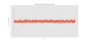
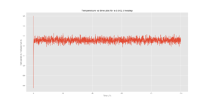
The 0.015 timestep diverges and is therefore unusable for further calculations as the accuracy would not be representative in the simulation relative to the real world. The 0.001 and 0.0025 timesteps converged to approximately the same energy, thus the 0.0025 timestep was used for future calculations as it strikes a balance between accuracy and computation time.

Correct choice of timestep for right reason. It would be good to add some intuition as to why larger timesteps cause the energy to diverge. What is happening from frame to frame that does not reflect reality?

TASK: Choose 5 temperatures (above the critical temperature $T^{*}=1.5$), and two pressures (you can get a good idea of what a reasonable pressure is in Lennard-Jones units by looking at the average pressure of your simulations from the last section). This gives ten phase points — five temperatures at each pressure. Create 10 copies of npt.in, and modify each to r Tick. un a simulation at one of your chosen $(p,T)$ points. You should be able to use the results of the previous section to choose a timestep. Submit these ten jobs to the HPC portal. While you wait for them to finish, you should read the next section.

Tick.

TASK: We need to choose $\gamma$ so that the temperature is correct $T=\mathfrak{𝔗}$ if we multiply every velocity $\gamma$. We can write two equations:

$\frac{1}{2}\sum _i{m}_i{v}_i^2=\frac{3}{2}N{k}_{B}T$

$\frac{1}{2}\sum _i{m}_i{\left(\gamma v_i\right)}^2=\frac{3}{2}N{k}_B\mathfrak{𝔗}$

Solve these to determine $\gamma$.

$\frac{\frac{1}{2}\sum _i{m}_i{v}_i^2=\frac{3}{2}N{k}_{B}T}{\frac{1}{2}\sum _i{m}_i{\left(\gamma v_i\right)}^2=\frac{3}{2}N{k}_B\mathfrak{𝔗}}$

$\frac{1}{{\gamma }^2}=\frac{T}{\mathfrak{𝔗}}$

$\gamma =\sqrt{\frac{\mathfrak{𝔗}}{T}}$

TASK: Use the manual page to find out the importance of the three numbers 100 1000 100000. How often will values of the temperature, etc., be sampled for the average? How many measurements contribute to the average? Looking to the following line, how much time will you simulate?

Nevery = 100

Nrepeat = 1000

Nfreq = 100000

Nevery samples the data every 100 timesteps (as defined).

Nrepeat averages the sample data every 1000 timesteps (as defined).

Nfreq is the average of the average of the sampled data every 100000 timesteps (as defined).

In this simulation LAMMPS averages the entire dataset (100000 timesteps, 250 for a 0.0025 timestep). So all the measuremants are taken into account in the average.

Tick

TASK: When your simulations have finished, download the log files as before. At the end of the log file, LAMMPS will output the values and errors for the pressure, temperature, and density $\left(\frac{N}{V}\right)$. Use software of your choice to plot the density as a function of temperature for both of the pressures that you simulated. Your graph(s) should include error bars in both the x and y directions. You should also include a line corresponding to the density predicted by the ideal gas law at that pressure. Is your simulated density lower or higher? Justify this. Does the discrepancy increase or decrease with pressure?

see above. Tick

TASK: As in the last section, you need to run simulations at ten phase points. In this section, we will be in density-temperature $({\rho }^{*},T^{*})$ phase space, rather than pressure-temperature phase space. The two densities required at $0.2$ and $0.8$, and the temperature range is $2.0,2.2,2.4,2.6,2.8$. Plot $C_V/V$ as a function of temperature, where $V$ is the volume of the simulation cell, for both of your densities (on the same graph). Is the trend the one you would expect? Attach an example of one of your input scripts to your report.

see above. There's a bit of a misunderstanding here - between the inherent chemical properties of a system and what changing these properties would mean for the heat capacity and simulating the heat capacity over our simulation of Lennard-Jones particles. In our simulation, and what I've tried to get people previously to suggest, we see a slight decrease in heat capacity with increasing temperature. What do we expect? Constant number of particles.. Internal enegy remains constant.. Cv = dU/dT and thus constant heat capacity. If I changed the material or the particles and changed the DOS or inherent properties of the systme, the heat capacity would vary as you suggest. INPUT SCRIPT:

### DEFINE SIMULATION BOX GEOMETRY ###
variable D equal 0.2
lattice sc ${D}
region box block 0 15 0 15 0 15
create_box 1 box
create_atoms 1 box

### DEFINE PHYSICAL PROPERTIES OF ATOMS ###
mass 1 1.0
pair_style lj/cut/opt 3.0
pair_coeff 1 1 1.0 1.0
neighbor 2.0 bin

### SPECIFY THE REQUIRED THERMODYNAMIC STATE ###
variable T equal 2.0
variable timestep equal 0.0025

### ASSIGN ATOMIC VELOCITIES ###
velocity all create ${T} 12345 dist gaussian rot yes mom yes

### SPECIFY ENSEMBLE ###
timestep ${timestep}
fix nve all nve

### THERMODYNAMIC OUTPUT CONTROL ###
thermo_style custom time etotal temp press
thermo 10

### RECORD TRAJECTORY ###
dump traj all custom 1000 output-1 id x y z

### SPECIFY TIMESTEP ###

### RUN SIMULATION TO MELT CRYSTAL ###
run 10000
unfix nve
reset_timestep 0

### BRING SYSTEM TO REQUIRED STATE ###
variable tdamp equal ${timestep}*100
fix nvt all nvt temp ${T} ${T} ${tdamp}
run 10000
reset_timestep 0

### MEASURE SYSTEM STATE ###
unfix nvt
fix nve all nve
thermo_style custom etotal temp atoms vol
variable temp equal temp
variable temp2 equal temp*temp
variable etotal equal etotal
variable etotal2 equal etotal*etotal
variable atoms equal atoms
variable vol equal vol
fix aves all ave/time 100 1000 100000 v_temp v_temp2 v_etotal v_etotal2
run 100000

variable avetemp equal f_aves[1]
variable avetemp2 equal f_aves[2]
variable aveetotal equal f_aves[3]
variable aveetotal2 equal f_aves[4]
variable heatcap equal (${atoms}*${atoms}*(${aveetotal2}-(${aveetotal}*${aveetotal})))/${avetemp2}


print "Averages"
print "--------"
print "Temperature: ${avetemp}"
print "Heatcap: ${heatcap}"
print "Volume: ${vol}"

TASK: perform simulations of the Lennard-Jones system in the three phases. When each is complete, download the trajectory and calculate $g(r)$ and $\int g(r)\mathrm{d}r$. Plot the RDFs for the three systems on the same axes, and attach a copy to your report. Discuss qualitatively the differences between the three RDFs, and what this tells you about the structure of the system in each phase. In the solid case, illustrate which lattice sites the first three peaks correspond to. What is the lattice spacing? What is the coordination number for each of the first three peaks?

P=N/V with P=1.2, N=4 (fcc unit cell), the lattice spacing is 1.494.

Lattice spacing is correct. See above for other feedback.

TASK: make a plot for each of your simulations (solid, liquid, and gas), showing the mean squared displacement (the "total" MSD) as a function of timestep. Are these as you would expect? Estimate $D$ in each case. Be careful with the units! Repeat this procedure for the MSD data that you were given from the one million atom simulations.

See above.

The extension velocity autocorrelation function tasks were not attempted.

References

- ↑ D. C. Rapaport and D. C., The art of molecular dynamics simulation, Cambridge University Press, 1995.
- ↑ M. Karplus and J. Kuriyan, Proc. Natl. Acad. Sci. U. S. A., 2005, 102, 6679–85
- ↑ Pang, YP. J Mol Model (1999) 5: 196.
- ↑ http://lammps.sandia.gov/
- ↑ http://www.ks.uiuc.edu/Research/vmd/
- ↑ J.-P. Hansen and L. Verlet, Phys. Rev., 1969, 184, 151–161.
- ↑ P. Atkins and J. De Paula, Atkins’ Physical chemistry 9th edition, 2009.
- ↑ J. Cohn, J. Phys. Chem., 1968, 72, 608–616.