Rep:AL1913

Introduction to molecular dynamics simulation

Velocity Verlet Algorithm

The velocity verlet algorithm is being used to model the behavior of the classical harmonic oscillator. The file related to the Velocity-verlet algorithm and relating it to the classical harmonic oscillator is found here

The analytic section relies on $x(t)=A\cos (\omega t)$

Figure 1: Graphs showing displacement, energy and the error against time for a time step of 0.1 seconds.

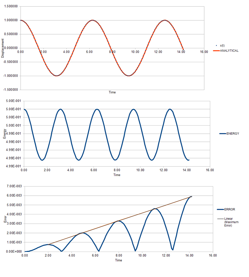
The position and potential energy agree with the harmonic oscillator model which is not too shocking due to the Verlet algorithm using Hooke's Law ($F=-kx$).

However, from the bottom plot, the absolute error of the system increases over the oscillations. As can be seen by the graph above, this is a linear plot implying that the algorithm carries errors forward from previous oscillations.

Figure 2: Graph showing how the total error increases with increasing size of the timestep

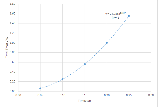
It was seen from the graph above that the smaller the timestep, the smaller the error. When the timestep is 0.20, the error was 0.1 % meaning that the any timestep below 0.20 will give an error less than 0.1 %. The first law of thermodynamics states that energy must be conserved and hence the total energy of an isolated system must be conserved. This means that the system with the smaller error in the energy will be the most accurate state of the ensemble.

Atomic Forces

Using the single Lennard-Jones potential interaction, the separation can be found where the potential energy is zero. The working out is shown below.

$\varphi (r)=4ϵ(\frac{{\sigma }^{12}}{r^{12}}-\frac{{\sigma }^6}{r^6})$

$0=4ϵ(\frac{{\sigma }^{12}}{r_0^{12}}-\frac{{\sigma }^6}{r_0^6})$

$\frac{{\sigma }^6}{r_0^6}=\frac{{\sigma }^{12}}{r_0^{12}}$

$r_0^6={\sigma }^6$

$r_0=\sigma$

Using the single Lennard-Jones potential interaction, the equilibrium separation can be found and using this the well depth can be found. The working out is shown below.

$\varphi (r)=4ϵ(\frac{{\sigma }^{12}}{r^{12}}-\frac{{\sigma }^6}{r^6})$

$\mathbf{F}=-\frac{\mathrm{d}\varphi (\mathbf{r})}{\mathrm{d}\mathbf{r}}$

$\mathbf{F}=4ϵ(\frac{-12{\sigma }^{13}}{r_{eq}^{12}}+\frac{6{\sigma }^7}{r_{eq}^7})=0$

$2{\sigma }^6=r_{eq}^6$

$r_{eq}=2^{\frac{1}{6}}\sigma$

$\varphi (2^{\frac{1}{6}}\sigma )=4ϵ(\frac{{\sigma }^{12}}{2^2{\sigma }^{12}}+\frac{{\sigma }^6}{2{\sigma }^6})$

$\varphi (r_{eq})=-ϵ$

The following integrals are considered and have been worked out in a similar way. The working out is shown below.

$\underset{2\sigma }{\overset{\mathrm{\infty }}{\int }}\varphi \left(r\right)\mathrm{d}r=4ϵ[\frac{{\sigma }^{12}}{-11r^{11}}+\frac{{\sigma }^6}{5r^5}{]}_{2\sigma }^{\mathrm{\infty }}$

When $\sigma =ϵ=1.0\underset{2\sigma }{\overset{\mathrm{\infty }}{\int }}\varphi \left(r\right)\mathrm{d}r=-0.024822443$

$\underset{2.5\sigma }{\overset{\mathrm{\infty }}{\int }}\varphi \left(r\right)\mathrm{d}r=4ϵ[\frac{{\sigma }^{12}}{-11r^{11}}+\frac{{\sigma }^6}{5r^5}{]}_{2.5\sigma }^{\mathrm{\infty }}$

When $\sigma =ϵ=1.0\underset{2.5\sigma }{\overset{\mathrm{\infty }}{\int }}\varphi \left(r\right)\mathrm{d}r=-0.008176748$

$\underset{3\sigma }{\overset{\mathrm{\infty }}{\int }}\varphi \left(r\right)\mathrm{d}r=4ϵ[\frac{{\sigma }^{12}}{-11r^{11}}+\frac{{\sigma }^6}{5r^5}{]}_{3\sigma }^{\mathrm{\infty }}$

When $\sigma =ϵ=1.0\underset{3\sigma }{\overset{\mathrm{\infty }}{\int }}\varphi \left(r\right)\mathrm{d}r=-0.003290128$

Periodic Boundary Conditions

The density of water is 1.0 g/mL, the molar mass of water is 18.01 g/mol. The moles of water per mL can be found by doing $\frac{1.0\text{ g/mL}}{18.01\text{ g/mol}}$. This number can be multipled by Avogadro's number to give the number of molecules per mL. There are 3.343 x 10²² molecules in one mL.

Using this number, the volume that 10000 molecules take up can be found. $\frac{10000}{3.343\times 10^{22}{\text{ mL}}^{-1}}=\mathbf{2}\mathbf{.}\mathbf{9}\mathbf{9}\mathbf{\times }\mathbf{1}{\mathbf{0}}^{\mathbf{-}\mathbf{1}\mathbf{9}}\text{ mL}$

If an atom starts at position (0.5, 0.5, 0.5) and moves (0.7, 0.6, 0.2) in a single step, the atoms ends up in (0.2, 0.1, 0.7) due to the periodic boundary condition of the box the atom is in. In vector form, this is shown below. $$\begin{gathered} \left[\begin{array}{c}0.5+0.7\delta \text{t}\\ 0.5+0.6\delta \text{t}\\ 0.5+0.2\delta \text{t}\end{array}\right]=\left[\begin{array}{c}1.2 \\ \\ 1.1\\ 0.7\end{array}\right]=\left[\begin{array}{c}0.2\\ 0.1\\ 0.7\end{array}\right] \end{gathered}$$

Given that $r^{*}=\frac{r}{\sigma }$ , that r* = 3.2 and $\sigma$ = 0.34 nm , it can be found that r = 1.088 nm.

As the well depth, $E_{welldepth}=-ϵ$, in reduced units,$E_{welldepth}^{*}=-1$

$E_{welldepth}=E_{welldepth}^{*}\times (\frac{ϵ}{k_B})\times k_B$

Given that $\frac{ϵ}{k_B}=120$:

$E_{welldepth}=-1\times 120\times 1.38\times 10^{-23}=1.66\times 10^{-21}J$

This can be multiplied by Avogardo's number and the Joules part can be converted to kilojoules:

$E_{welldepth}=1.00kJmo{l}^{-1}$

Given that $T^{*}=\frac{k_{B}T}{ϵ}$ , that T* = 1.5 and that $\frac{ϵ}{k_B}=120$, it can be found that $T=180K.$

Equilibration

Creating the simulation box

A system could initially start with a very high energy system if two atoms are close together as the potential energy would be very high. They would move away from each other with a very high velocity with the system having an improbably high energy.

Figure 3: Face Centred Cubic Lattice Plan

There is one atom per unit cell. The volume of the unit cell can be found by calculating $\frac{\text{atoms per unit cell}}{\text{number density}}$. The length can be found by taking this result and taking it to the power of a third. Hence for a simple cubic lattice with a density of 0.8, length = $(\frac{1}{0.8}{)}^{\frac{1}{3}}=1.07722$

The number of atoms per unit cell for a face centered cubic lattice is 4 ($\frac{1}{8}\times 8+\frac{1}{2}\times 6$). The length of this cubic unit cell is $(\frac{4}{1.2}{)}^{\frac{1}{3}}=1.49$

The create_atoms command would make 4000 atoms; 4 atoms per unit cell with 1000 unit cells being produced.

Setting the properties of the atoms

mass 1 1.0
pair_style lj/cut 3.0
pair_coeff * * 1.0 1.0

The mass of atom 1 is set to be 1.0 pair_style sets the type of energy interactions between each pair of atoms, which in this case is the Lennard-Jones potential with any interactions beyond $3\sigma$ being discounted. The pair_coeff relates to $ϵ$ and $\sigma$ respectively. The * * means these are considered for the whole system, with 1.0 1.0 meaning the values of these are 1.0.

Given that we are specifying ${\mathbf{x}}_i\left(0\right)\text{and }{\mathbf{v}}_i\left(0\right)$, the velocity Verlet algorithm is going to be used.

Running the simulation

By considering the lines below, the code can be understood quite easily.

### SPECIFY TIMESTEP ###
variable timestep equal 0.001
variable n_steps equal floor(100/${timestep})
variable n_steps equal floor(100/0.001)
timestep ${timestep}
timestep 0.001

The first line defines the timestep used, which is 0.001 in this case.
The duration of the simulation is kept constant, with 100 time units being used in this case.
### RUN SIMULATION ###
run ${n_steps}
run 100000

We can not just write:

timestep 0.001
run 100000

This set of codes requires the changing of all lines related to timestep manually if the timestep is to be changed.

In the first code, the modifications can be made more easily.

Checking equilibrium

Figure 4: Graph showing how the total emergy changes with timestep

Figure 5: Graph showing the pressure changes with time for the 0.0001 timestep

Figure 6: Graph showing the temperature changes with time for the 0.0001 timestep

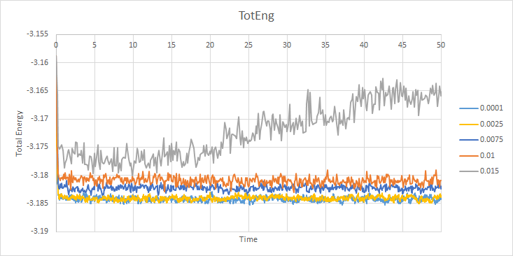
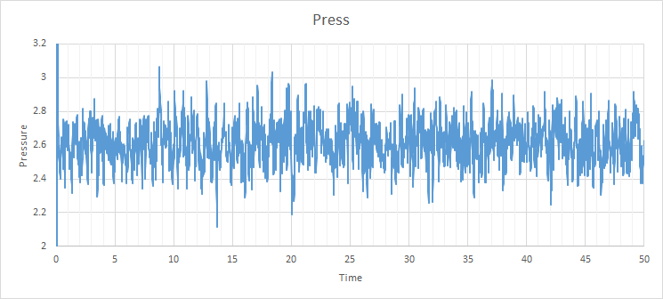
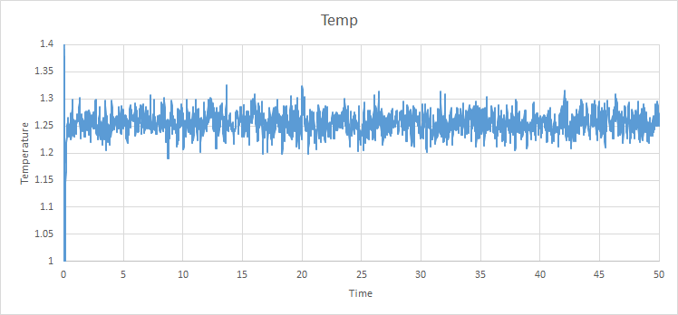
For the 0.001 timestep, the system reaches the equilibrium state within 0.25 seconds (250 timesteps) This is also the same for the pressure and temperature seen below. The largest of the timesteps to give reasonable results for the energy is 0.01 seconds. However, the largest result with the lowest energy is 0.0025 seconds, so it is the best to be used for finding subsequent results. The poorest result is 0.015 seconds for each timestep as the simulation does not reach equilibrium, which is impossible due to the first law of thermodynamics.

Running simulations under specific conditions

Thermostats and Barostats

By using the following two equations, a relationship for $\gamma$ can be found.

$\frac{1}{2}\sum _i{m}_i{v}_i^2=\frac{3}{2}N{k}_{B}T$

$\frac{1}{2}\sum _i{m}_i{\left(\gamma v_i\right)}^2=\frac{3}{2}N{k}_B\mathfrak{𝔗}$

$\frac{\sum _i{m}_i{v}_i^2}{\sum _i{m}_i{\left(\gamma v_i\right)}^2}=\frac{T}{\mathfrak{𝔗}}$

$\frac{\sum _i{m}_i{v}_i^2}{{\gamma }^2\sum _i{m}_i{v}_i^2}=\frac{T}{\mathfrak{𝔗}}$

$\gamma =\sqrt{\frac{\mathfrak{𝔗}}{T}}$

Examining the Input Script

### MEASURE SYSTEM STATE ###
thermo_style custom step etotal temp press density
variable dens equal density
variable dens2 equal density*density
variable temp equal temp
variable temp2 equal temp*temp
variable press equal press
variable press2 equal press*press
fix aves all ave/time 100 1000 100000 v_dens v_temp v_press v_dens2 v_temp2 v_press2
run 100000

The importance of the three numbers 100 1000 100000 in the input script need to be considered.

The importance of the number 100 is that the input values are used every 100 timesteps. The importance of the number 1000 is that it is the number of times to use the input values to calculate averages. The importance of the number 10000 is the number of timesteps it takes to calculate the averages. Every 10000 steps, the average will be sampled. 1000 steps will contribute to the average. It will run for 10000 steps for the simulations.

Plotting the Equations of State

Figure 7: Graph showing how the density changes with temperature for different densities, with simulated and ideal gas conditions considered

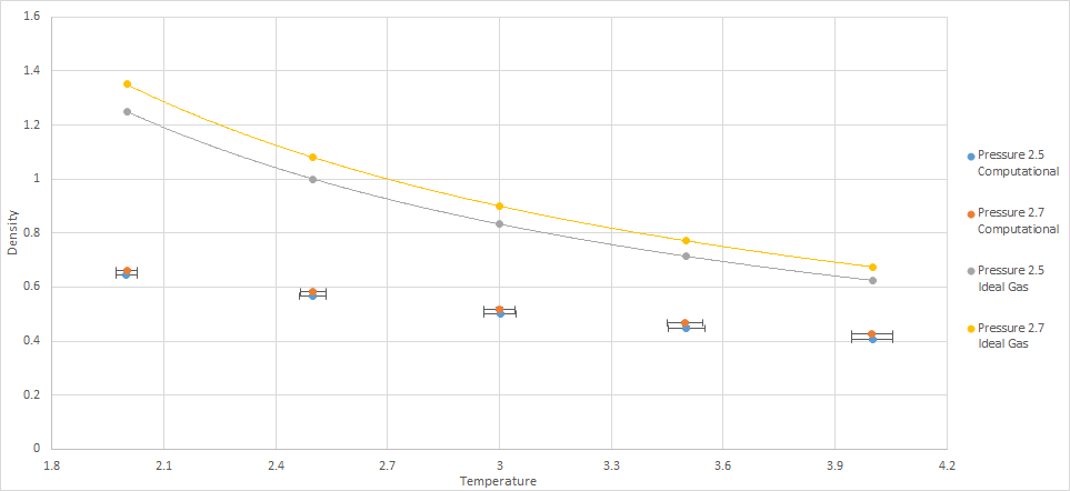
The simulated density is much lower than that predicted by the ideal gas law. The ideal gas law assumes that there is no interaction between gas molecules. This means that the molecules can approach each other, even to very small distances, with no penalty. The discrepancy decreases as the temperature increases. The ideal gas law implies that as T approaches zero, the density can approach infinity. In the simulation, using Lennard-Jones potential, this is not possible as the atoms cannot approach each other as easily due to the high potential energy caused by the nuclei approaching too closely. The discrepancy increases as pressure increases. Molecules will experience a larger repulsive force as the molecules are closer together and so the density will be lower. Due to the ideal gas law not taking these forces into account, the discrepancy increases as pressure increases.

Calculating heat capacities using statistical physics

Figure 8: Graph showing how the heat capacity changes with temperature for different densities, with simulated conditions considered

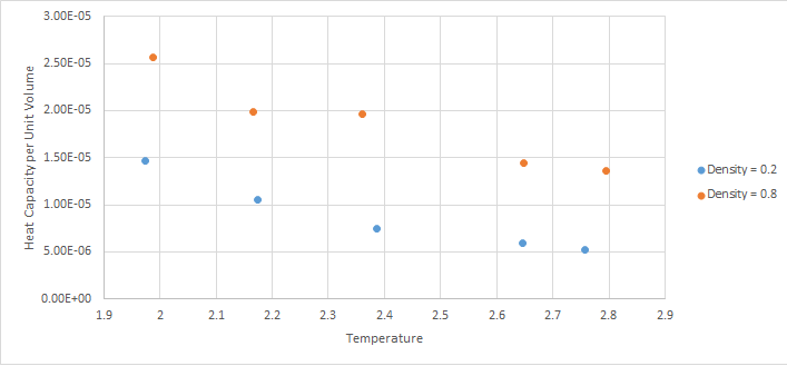
As the temperature increases, the heat capacity decreases. $C_V=\frac{dQ}{dT}$ so it would be expected that if Q was not dependent on T than it would stay constant. This is not the case as can be seen by the graph and so as T increases, Q must decrease leading to the graph shown.

At higher densities, the heat capacity per unit volume increases. This means the heat capacity increases with the number of atoms. This is expected because the heat capacity is an extensive property therefore it is proportional to the size of the system.

An input file for the density at 0.2 and temperature at 2.0 is provided here

Structural properties and the radial distribution function

The radial distribution function (RDF), g(r), describes how the density of particles varies as a function of distance from a reference particle.

Figure 9: Graph showing how the RDF changes with distance for a specific atom for different states

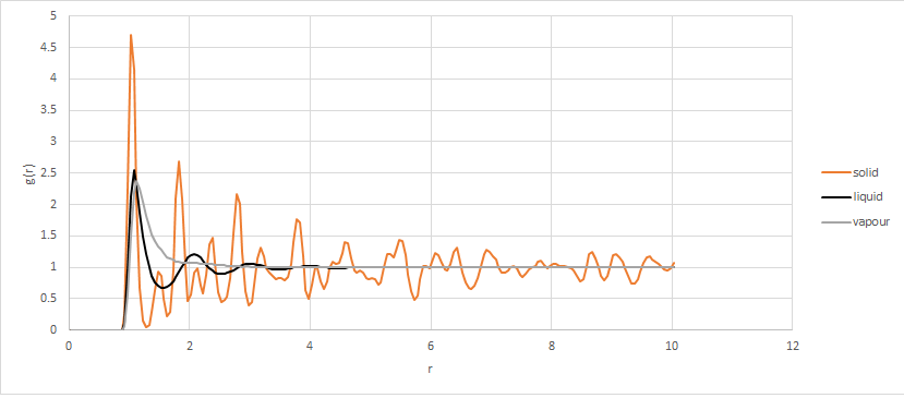
Between the value of r = 0 to 0.825, all of the RDF graphs have a value of 0. This is due to repulsive forces dominating in this region.

When g(r) approaches 1, it means there are no significant numbers of atoms found and so no predictable arrangement of atoms at this distance.

The RDF graphs oscillate around the value of 1. The solid oscillates for a longer distance than the liquid. At the peaks of the graphs, atoms will be found. This suggests that the solid has a more ordered structure which are packed more closely.

In the liquid there are a few peaks which are further apart, with no more oscillations after 4 units with g(r) approaching 1. In the vapour, there is one peak prior to 2 units with g(r) approaching 1 after this point. This suggests that the liquid has atoms further apart than the solid and the gas has atoms further apart than the liquid, and so solid. Another way of putting this is that the solid has the most atomic shells and the gas has the least atomic shells in a given distance.

The Solid Lattice

By using the face-centred lattice and a number density of 0.8 the length of one side of the unit cell is 1.49. The peaks of the solid RDF have been found to give the distance of the nearest neighbours. The integration of each peak gives the coordination number of that atom.

Figure 10: Graphs showing how the RDF and integrated RDF changes with distance for a specific atom for the solid state

Figure 11: Diagram showing the three nearest neighbours from the specified atom [red] (Black is the nearest neighbour. Blue is the 2nd nearest neighbour. Green is the 3rd nearest neighbour).

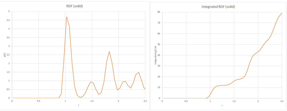
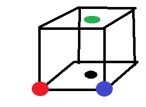
Red is the atom specified in this case, Black is the nearest neighbour. Blue is the 2nd nearest neighbour. Green is the 3rd nearest neighbour.

Distance	Comparison to unit,cell length (A)	Integration Values (nearest whole number) of Troughs beside peak	Coordination Number
1.025	Approximately,$\frac{1}{2^{0.5}}A$	0 and 12	12
1.475	Approximately A	12 and 18	6
1.825	Approximately$\frac{6^{0.5}}{2}A$	18 and 42	24

More distances in this region need to be solved for this to be more accurate, hence leading to slight inaccurate results being produced.

Dynamical properties and the diffusion coefficient

Mean Squared Displacement

The atoms follow Brownian motion which is random meaning the position probability density diffuses out over time. Brownian motion would only be expected for liquid and gaseous systems and hence a non-zero diffusion coefficient in liquid and gaseous systems is also expected.

Figure 12: Graph showing how the MSD changes with distance for a specific timestep [0.002 s] for the three states with 8000 atoms and a million atoms considered

The graphs shown do not use time but rather the number of time steps. Hence D = 1/6 x gradient x 1/time step for these graphs. The time step used is 0.002 s. The gradient is only found for the region where the graph seems to be a straight line. For the gaseous MSD functions there is an initial non-linear relationship due to the atoms’ initial velocity dominate the function before collisions with other atoms lead to the linear function to dominate. The higher density of liquid lead to this non-linear region to be much smaller, so much so that it is unnoticeable in this work. As reduced units are used for the distance, the units of D in this case is s^-1.

D ($s^{-1}$)	8000 atoms	Million Atoms
Solid	$-2.31091\times 10^{-6}$	$-8.76319\times 10^{-6}$
Liquid	$0.083165173$	$0.087264304$
Gas	$2.85910032$	$3.015986882$

The solid has a slight non-zero value due to slight errors which would be caused by not using a long enough timeframe. The million atom systems has higher diffusion constants than the 8000 atom systems.

Velocity Autocorrelation Function

The evaluation of the normalised velocity autocorrelation function for a 1D harmonic oscillator is shown below:

$C\left(\tau \right)=\frac{\underset{-\mathrm{\infty }}{\overset{\mathrm{\infty }}{\int }}v\left(t\right)v(t+\tau )\mathrm{d}t}{\underset{-\mathrm{\infty }}{\overset{\mathrm{\infty }}{\int }}{v}^2\left(t\right)\mathrm{d}t}$

$x\left(t\right)=A\cos (\omega t+\varphi )$

$v\left(t\right)=-A\omega \sin (\omega t+\varphi )$

$v(t+\tau )=-A\omega \sin (\omega (t+\tau )+\varphi )$

$C\left(\tau \right)=\frac{\underset{-\mathrm{\infty }}{\overset{\mathrm{\infty }}{\int }}-A\omega \sin (\omega t+\varphi )\times -A\omega \sin (\omega (t+\tau )+\varphi )\mathrm{d}t}{\underset{-\mathrm{\infty }}{\overset{\mathrm{\infty }}{\int }}(-A\omega {)}^2{\sin }^2(\omega t+\varphi )\mathrm{d}t}$

$C\left(\tau \right)=\frac{\underset{-\mathrm{\infty }}{\overset{\mathrm{\infty }}{\int }}{A}^2{\omega }^2\sin (\omega t+\varphi )\sin (\omega t+\omega \tau +\varphi )\mathrm{d}t}{\underset{-\mathrm{\infty }}{\overset{\mathrm{\infty }}{\int }}{A}^2{\omega }^2{\sin }^2(\omega t+\varphi )\mathrm{d}t}$

Let $\alpha =\omega t+\varphi$ and $\beta =\omega \tau$

$C\left(\tau \right)=\frac{\underset{-\mathrm{\infty }}{\overset{\mathrm{\infty }}{\int }}\frac{1}{\omega }\sin \left(\alpha \right)\sin (\alpha +\beta )\mathrm{d}\alpha }{\underset{-\mathrm{\infty }}{\overset{\mathrm{\infty }}{\int }}\frac{1}{\omega }{\sin }^2\left(\alpha \right)\mathrm{d}\alpha }$

$C\left(\tau \right)=\frac{\underset{-\mathrm{\infty }}{\overset{\mathrm{\infty }}{\int }}\sin \left(\alpha \right)\sin \left(\alpha \right)\cos \left(\beta \right)+\sin \left(\alpha \right)\cos \left(\alpha \right)\cos \left(\beta \right)\mathrm{d}\alpha }{\underset{-\mathrm{\infty }}{\overset{\mathrm{\infty }}{\int }}{\sin }^2\left(\alpha \right)\mathrm{d}\alpha }$

$C\left(\tau \right)=\frac{\underset{-\mathrm{\infty }}{\overset{\mathrm{\infty }}{\int }}{\sin }^2\left(\alpha \right)\cos \left(\beta \right)\mathrm{d}\alpha }{\underset{-\mathrm{\infty }}{\overset{\mathrm{\infty }}{\int }}{\sin }^2\left(\alpha \right)\mathrm{d}\alpha }+\frac{\underset{-\mathrm{\infty }}{\overset{\mathrm{\infty }}{\int }}\sin \left(\alpha \right)\cos \left(\alpha \right)\sin \left(\beta \right)\mathrm{d}\alpha }{\underset{-\mathrm{\infty }}{\overset{\mathrm{\infty }}{\int }}{\sin }^2\left(\alpha \right)\mathrm{d}\alpha }$

$C\left(\tau \right)=\cos \left(\beta \right)+\frac{\sin \left(\beta \right)\underset{-\mathrm{\infty }}{\overset{\mathrm{\infty }}{\int }}\sin \left(\alpha \right)\cos \left(\alpha \right)\mathrm{d}\alpha }{\underset{-\mathrm{\infty }}{\overset{\mathrm{\infty }}{\int }}{\sin }^2\left(\alpha \right)\mathrm{d}\alpha }$

$C\left(\tau \right)=\cos \left(\beta \right)+\frac{\frac{1}{2}\sin \left(\beta \right)\underset{-\mathrm{\infty }}{\overset{\mathrm{\infty }}{\int }}\sin \left(2\alpha \right)\mathrm{d}\alpha }{\frac{1}{2}\underset{-\mathrm{\infty }}{\overset{\mathrm{\infty }}{\int }}1-\cos \left(2\alpha \right)\mathrm{d}\alpha }$

$\underset{-\mathrm{\infty }}{\overset{\mathrm{\infty }}{\int }}\sin \left(2\alpha \right)\mathrm{d}\alpha =0$ due to symmetry of the function.

So $C\left(\tau \right)=\cos \left(\beta \right)=\cos \left(\omega \tau \right)$

Figure 13: Graph showing how the VACF changes with $\tau$ for a specific timestep [0.002 s] for the three states with 8000 atoms (bottom) and a million atoms (top) considered

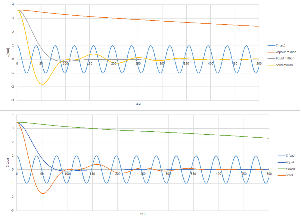
As can be seen by the graph, the simulated system differs majorly from the harmonic oscillator velocity autocorrelation function (VACF). There is damping evident in the simulated systems, where the gaseous system is significantly damped and the solid system is the least damped of the three states. The harmonic oscillator does not take into account this damping. This is due to the lack of potential energy with relation to other atoms in the system. The gaseous state is less viscous than the liquid state which means the gaseous system needs more time for atoms to collide with each other, as there are less atoms per unit volume and so more time is needed correlate the velocity. The liquid state has more collisions within the same time than the gas state meaning the velocity correlates much more quickly. It ‘overshoots’ slightly which is likely due to some inertia from the initial system conditions. The solid is most similar to the harmonic oscillator due to the atoms’ positions being well defined. Any change to this position is corrected more quickly due to the highly sensitive distance dependent in the solid state. It does dampen however.

As the gaseous does not reach a stable value, D cannot be found in this case. The solid will be assumed to have reached a stable value after 1000 time steps. The liquid seemed to be stable by 150 time steps. Again, the number of time steps were used, but this time it was a product and so the time step (0.002 s) should be multiplied with the trapezium rule guesses.

Figure 14: Graphs showing how the intergrated VACF changes with $\tau$ for a specific timestep [0.002 s] for the three states with 8000 atoms (right) and a million atoms {left) considered using a running trapezium rule

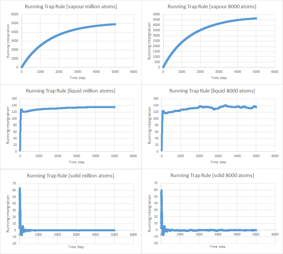
D (s)	8000 atoms	Million Atoms
Solid	$4.77\times 10^{-5}$	$-5.07\times 10^{-4}$
Liquid	$0.0790$	$0.809$
Gas	-	-

The biggest source of error in estimating D is that the convergence must be guessed by eye. The actual convergence may take much longer. Furthermore, the random motion of the atoms lead to oscillations which may be significant to the integral.