Introduction to molecular mechanics and force fields

History of Molecular Modelling and Molecular Mechanics

The origins of the molecular mechanics method can be traced to work done by Barton in the late 1940s, as well as Bright-Wilson (Molecular Vibrations, 1938. DOI: 10.1063/1.1750232) and others in the late 1940s and early 1950s and e.g. Allinger (starting in 1959, DOI: 10.1021/ja01530a049) and the MM2/3/4 force fields and Kollman/Amber in the 1970s-80s.

The Force Field

The steric energy of a molecule is defined by the following terms (normally five, but can be more). These terms are independent, and each relate to transferable properties of molecules. The constants in these equations together constitute what is called a mechanics force field (notice how there are no terms relating to electrons, apart from being implied in the charges q_i on the atoms!).

$E_{s t e r i c} = \sum_{b o n d s} K_{r} (r - r_{e q})^{2} + \sum_{a n g l e s} K_{θ} (θ - θ_{e q})^{2} + \sum_{d i h e d r a l s} \frac{V_{n}}{2} [1 + c o s (n ϕ - γ)]$ $+ \sum_{n o n - b o n d e d} [\frac{A_{i j}}{R_{i j}^{12}} - \frac{B_{i j}}{R_{i j}^{6}} + \frac{q_{i} q_{j}}{ϵ R_{i j}}] + \sum_{H - b o n d e d} [\frac{C_{i j}}{R_{i j}^{12}} - \frac{D_{i j}}{R_{i j}^{10}}]$

These five equations have the following meanings:

A quadratic function
The bond stretching term, defined by a quadratic function, where K is the bond force constant.
the bond angle term, also a quadratic function.
the dihedral term, describing the torsion around a bond; low for a single and triple bond, high for a double bond, medium for a delocalized bond. V is related to the barrier for rotation about the bond.
the non-bonded term, split into two components:
1. The 6-12 potential, which describes the dispersion interactions between atoms, and which can be both repulsive (1/r¹²) and attractive (/r⁶).
2. The elecrostatic term, for which charges on individual atoms must be assigned, and which again can either attract or repel depending on whether each pair of charges opposes or attracts.
An (often optional) hydrogen bond term.

Characteristic Properties

The force field resulting from these equations has a number of characteristic properties:

The steric energy is normalised relative to zero (for the first three terms), rather than to any thermodynamic quantity.
The parameters in the above equations require definition of the atom types which in turn impacts upon the bond and angle types.
- For lengths, each parameter (force constant) is specific to the particular atom pair. If you think about it, a great many different atom pair combinations are possible from the 70+ elements of the periodic table that you might want to model. Few force fields have even a fraction of these permutations.
- Things get even worse for the three atoms defining an angle.
- For the torsional term, no attempt is made to conver all permutations of four atoms; rather parameters are inserted merely for the common single and double bonds.
- The fourth term, which requires the charges on each atom pair is again approximated with various relatively crude charge schemes, often obtained from Quantum mechanical calculations.
- The hydrogen bonded term is considered as just between two specific atoms, and parameters for each atom pair combination have to be defined. Delocalized hydrogen bonds (e.g. to the face of an aryl group) are not covered.
- Some mechanics implementations insert cross-terms, ie stretch-bend. These are not normally large.
- Many (often proprietary) force fields include additional terms in the sum above, relating to
  - π-conjugation
  - Stereo-electronic (anomeric) effects, but in parametric form rather than wavefunction derived.
As an approximate rule of thumb, the first three terms in the above equation tend to zero for unstrained and unhindered molecules. A high positive value of the steric energy is therefore taken as an indication of instability. The fourth term can take on negative values, particularly if the molecule is globular (lots of non-bonded attractive terms) or if the molecule has many ionic interactions where qi and qj have opposite signs.
Two force fields implementing the above equations which you have access to are MM2 and MMFF94. There are many other, often specialized force fields.
There are also a so-called universal or full periodic table force field (UFF, DOI:10.1021/ja00051a040 DOI:10.1021/ja00051a040 ) where an attempt is made to interpolate atom pair or atom triple values from the basic hybridization specified for each atom, and specific values for each atom. These are not very good for energies, but suffice for cleaning up a crudely drawn structure. They can also be applied to many more elements of the periodic table than the MM2/3/4 style force fields.
Energies should be compared for isomers with the same total number of atom/bond types.
Energies should not be compared across different force fields (or indeed across different programs implementing apparently the same force field!)
The minima found are restricted to the "atom-connectivity" specified in the input file; no bonds can make/break during the optimisation process (and hence no matter how bad the initial geometry guess is, that connectivity will be preserved). But this also means that in general bond-breaking transition states cannot be located using Mechanics. Bond-rotating and angle-inverting transition states can be approximated however. This topic will be the subject of a separate lecture in this mini-series.
Mechanics is however prone to "false minima", allowed by the equations, but physically unrealistic (e.g. hemispherical carbon).
Force field parameters can be of widely differing quality
Mechanics can be very reliable for geometric predictions, and is the method of choice for interfacing between 2D/3D structure sketch programs, and expensive QM programs. Programs such as Avogadro implement perpetual force field optimisers, which operate even as you draw the molecule, resulting in an "elastic band" effect. You can distort the molecule by dragging one or more atoms away, and watch how the mechanics force field restores the geometry to equilibrium. However, do not confuse this with molecular dynamics, for which a quite different set of equations are solved.
Mechanics, when used with high quality parameter sets, can be very reliable for calculating vibrational properties (IR frequencies, but not intensities!).
Mechanics is good for conformational exploration (Monte-Carlo, Genetic algorithms, etc)
Mechanics is also highly applicable to molecular dynamics, and hence statistical thermodynamic quantities such as free energies etc (but this is not a part of the present course).

Summary of Pros and Cons of Molecular Mechanics

Pros: Simple energy functions are quick to solve, can cope with large molecules, accurate for systems which are close to the models used to reproduce the force field (interpolative), can be used to specify mandatory bonds in a molecule.

Cons: No unique function for each energy term, number of parameters rises rapidly for non CHNO elements, need to know atom/bond type for all the molecule, cannot cope with unusual bonding situations. Cannot be used for bond-breaking transition states.

Geometry Optimization

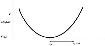
The process of optimizing a geometry involves application of the truncated Taylor Theorem expansion of the energy. By including only the first three terms, we are approximating the potential energy by a quadratic function. Since real surfaces are not quadratic, we have to iterate this simple procedure to convergence.

There are four ways of populating the inverse Hessian matrix:

Steepest_descent,, which sets the diagonal terms to 1, and all the others to zero. Very fast, particularly initially, and suitable for the largest molecules since no matrix inversion need be performed. An option in most mechanics methods.
Conjugate_gradient, which evaluates the value of only the diagonal terms, setting all the others to zero. Slower, but meanders less when the gradient is no longer "steep". Most mechanics methods implement this.
BFGS_method, which evaluates the diagonal terms, and approximates the off-diagonal terms from the history of the optimisation. Much slower, and less suitable for large molecules, since inverting the Hessian is now increasingly time consuming. Most Molecular orbital/DFT methods use this, or variations (thus the opt keyword in Gaussian) since in fact the bottleneck is not inverting the Hessian, but integral evaluations.
Newton-Raphson, which evaluates all the terms. Very slow, but can succeed when all other methods fail (opt(calcall) keyword in Gaussian!) and has gotten a lot easier now that really efficient 2nd derivative algorithms have been developed (e.g Gaussian 09).

The value of Δx is obtained from a one-dimensional line search to obtain a scaling factor (normally around 0.25, and which helps correct for the non-quadratic behaviour of the energy potential), and an iterative process started;

Calculate Δx at first guessed geometry.
Change geometry and recalculate Δx.

Convergence is achieved when either the value of Δx reaches a small predetermined value, or the change in energy between successive cycles becomes small.