Go to Introduction | Go to Workshops | Go to MatLab primer

First Year Data Analysis and Presentation 2012-2013 Workshops 2012

Two approaches to data analysis are demonstrated in this workshop; the first is the use of Microsoft Excel, and the second, more powerful option is to use MatLab.

Excel is a general purpose tool for analysing data with which you are likely to already be familiar. Its visual nature will allow you to easily see the operations you are performing and will provide you instant feedback on the changes you make. The majority of this class is devoted to Excel and to demonstrate some more advanced techniques with this spreadsheet package.

An introduction to MatLab is provided as it is a more powerful option, particularly for analysing large quantities of data - in Excel changes can only be performed one at a time, and if you have a great deal of data to analyse these tasks can rapidly become repetitive.

MatLab is NOT the main focus of the workshop, as we are focusing on techniques for data analysis rather than software for data analysis. You may find it useful to work through this MatLab primer in your personal study time as it may give you further perspective on data analysis, and will help you throughout your course of study in Physical and Computational Chemistry at Imperial College.

Assessment

DEADLINE - FRIDAY 30th NOVEMBER

The assessment for these workshops takes the form of a Blackboard assessment, followed by submission of your Excel spreadsheet/MatLab script/other relevant file. Each stage of the analysis will yield a numerical solution and you will be able to enter these into the appropriate Blackboard assessment for each stage of the workshop. You can submit the assessment at any time until the closing date. NOTE: Whichever software you wish to use to analyse your data, you must make sure it is clear how you obtained your results.

Completion of the assessment is a requirement for award of First Year Honours, however it is set up to allow you to monitor your own progress with the material to assess your own competency. Whether you use Excel or another program to analyse the data is up to you, but as long as you are familiar with the routes for data analysis you will have fulfilled the objectives of this course.

The assessments may be found within Blackboard; from the course home page, navigate to "Course Materials -> Summative Assignment".

Microsoft Excel

The built in 'Help' facility in Excel is excellent, and will provide ready assistance when finding formulae and functions. This should be your first port of call if you are looking for a solution. Failing that, you can always use a popular internet search engine. Demonstrators will be on-hand to help you during the workshop, but bear in mind that if they don't know the answers immediately, the chances are they will refer to one of these two resources also!

Quick hints and tips

The basics of mathematical formulae in Excel:

To type a mathematical expression, select a cell and type:

=3+5

Upon pressing <enter>, this equation should evaluate.

Other operators are detailed as follows:

+ - * / ( )

addition, subtraction, multiply, divide, brackets

To 'raise' a power (e.g. 4²), type the following:

=4^2

Pressing <enter> will then evaluate the cell.

Many operations in Excel involve taking a value from one cell and using it in a calculation elsewhere. This can either be done by typing:

=A5<function>

to apply a function to the contents of cell A2, or by typing "=" (no quotes) and then clicking on cell A5 then typing the function.

Constants

Some constants can be invoked simply:

Invoking Constants in Excel
Syntax in cell	Result
=PI()	$π$
=PI()*2	2 $π$
=EXP(2)	e²

...while others will need to be defined as part of your spreadsheet.

Standard Form, or Scientific notation

To enter a number in standard form in Excel the following syntax must be used:

Physical constants in standard form
Syntax in cell	Result
6.022E+23	Avogadro's number, 6.022 x 10²³
1.602E-19	Charge on an electron, 1.602 x 10^-19 C
6.626E-34	Planck's constant, 6.626 x 10^-34 m²kg s^-1

If you were to try and enter a very small value as 0.000000000000456, you may find that Excel simplifies it to 0!

Other handy hints


Typing formulae Formulae can be entered in Excel by typing "=" (no quotes) and then clicking on cells, together with the operators required (Figure 1). You will see that the cells will be colour-coded to match your formula. You can also type "=(B7*C7)/D7" and achieve the same results.	Figure 1
Setting a constant A constant can be set by keeping it separate from the main body of the data, in this instant the Gas Constant, R in cell E2 (Figure 2).	Figure 2
Evaluating Pressing <ENTER> will then evaluate the cell (Figure 3).	Figure 3
Applying to other values 1 Instead of typing the formula out again into other cells, you can place your mouse over the blue 'grab handle' in the bottom right of the cell (where the cursor will change), and drag it down through all the cells you want to apply the formula to (Figure 4).	Figure 4
Fixing the formulae 1 As you can see, there are errors in the evaluation (Figure 5). When formulae are extended in this way, they dynamically adapt to the changing row (and columns if you drag sideways) - so "(B7C7)/(D7E2)" becomes "(B8C8)/(D8E3)", "(B9C9)/(D9E4)" etc..	Figure 5
Fixing the formulae 2 Double-clicking a cell reveals its formula; as described above, the formula have dynamically adjusted (Figure 6). This is fine for B8, C8 and D8 - we need these to adjust, but we need to fix E2 so it doesn't change.	Figure 6
Fixing the constant In order to specify a cell which does not change, we need to use the "$" operator (Figure 7). Typing $E$2 will lock that cell in the formula and not allow its row or column to change; similarly $E7 will not allow its column to change, but the row number can vary, and E$7 will allow the column to vary, but lock the row number.	Figure 7
Applying to other values 1 If you now use the grab handle and drag downwards, you will then see all the formulae evaluating correctly (Figure 8). Double clicking on any cell will show the formula working as expected.	Figure 8
Fixing the constant 1 (alternate method) Another way to lock the constant cell in a formula is to name the cell. Clicking on the cell, then the Name box (circled, Figure 9), allows you to specify a name for that cell, in this case "GCR", but you can name it anything you need.	Figure 9
Fixing the constant 2 (alternate method) This name can then be used in the formula; double click the first cell and replace $E$2 with GCR; this will lock the cell and it can be 'dragged' as before (Figure 10).	Figure 10

Workshop exercises

The Standard Error

As discussed in lectures, the standard error is that which should be reported whenever you report a mean value. It is found using Equation 1 shown to the right.

In order to evaluate the standard error, you will need to evaluate the sample standard deviation using the equation shown in your lecture notes (and in MATU p13 - make sure you can identify the correct equation). Using Excel, the aim of this first task will be to identify the standard error in a series of measurements so that you can then make a report of the error in the mean value for each data series.

First steps

Ten data sets are available for analysis, the file containing these data sets may be downloaded from Blackboard. The first thing you will notice is the file type. This is not an ordinary Excel data file; rather this is what is termed a "CSV" file - a 'comma separated value' file. This is the standard text file which is exported by the majority of data-recorders and is readily accessible by almost every analysis program around. It can even be opened in Notepad/Textedit for your own viewing.

Right-click the downloaded file and select 'Open in Excel'
- If this option is not available, you can open excel, click File -> open and then navigate to where the file is saved.
This should open directly to give you a spreadsheet of values.

Analysing the first data set (column A):

Copy the first column (vertical set) into a new spreadsheet
First find the mean of the data values:
- in one of the cells below the data set type the following:

=(

...then select each of the cells, adding them together. Once done, type

)/10

You should have something that looks like the following:

=(A2+A3+A4+A5+A6+A7+A8+A9+A10+A11)/10

Press <ENTER> to evaluate.

This can be shortened as follows:

Select another cell below the first mean calculation, and type the following:

=(SUM(A2:A11))/10

...pressing <ENTER> to evaluate (if your cells are differently numbered, change the numbers accordingly). Instead of typing "A2:A11", you can simply 'click-and-drag' after you have typed "=(SUM(" , remembering to close your brackets after you have done so.

Notice the use of brackets to 'partition' parts of the formula to ensure that the expression evaluates correctly.

Finding the mean can be further shortened as follows:

Selecting a third cell below the first mean calculation, type the following

=AVERAGE(A2:A11)

...pressing <ENTER> to evaluate.

Many statistical operations have a dedicated function in Excel in this manner; you may wish to experiment with other average functions such as MODE and MEDIAN in this instance. Continuing with the standard error determination, we now need to find the sample standard deviation, s:

In the adjacent column (if your data is in column A2:A11, use column B) you will set up your 'residuals squared' (you may wish to put an appropriate label into cell B1). We will assume that your mean value has been determined and lies in cell A12
Clicking cell B2, apply the following formula:

=(A2-A$12)^2

...remembering to use the "$" operator to fix the row number of your mean, and to correct it from A12 if your mean is in a different cell. This will determine your residual and square it (the "^" symbol denoting a power). Click and drag the cell down to apply this to the rest of the column. You will then want to sum this value underneath the column.

You now have the sum of the squared residuals. According to the sample standard deviation formula there are only a few more operations to perform; divide this value by (N-1), and then find the square root.

Use the Excel help file to locate the square root function and how to use it. This will then give you your sample standard deviation.

Finding the standard error is now a trivial matter as shown in Equation 1 above.

Take your standard deviation, and divide it by the square root of the population size. Make note of this value.

Analysing the second data set

Now that we have set up the spreadsheet, we can now analyse the second data set slightly quicker.

Copy the second data set and paste it into Column D (leaving a space where column C is will keep things from becoming confused)
Copy your mean calculations from below Data Set 1 in Column A, and paste into the same rows in Column D.
- You should find that the values adjust to the new data set! Double clicking one of these cells will reveal its formula - by default Excel copies the formula, not the values. To paste values only, right-click and select "Paste Special".
Copy the cells from Column B, and paste into Column E; again the values should update, and you will be able to see your standard error and standard deviation immediately.
Make a note of your standard error value.

Analysing the other data sets

In theory, you could just carry this on to analyse all ten data sets, however the spreadsheet will start to look very cluttered very quickly. Instead, we're going to use the power of Excel to do a lot of the work for us.

Copy and paste the remaining data sets into a new spreadsheet
- You may find it useful to leave Column A blank in order to put labels into it
Select a cell underneath Set 3 in which to calculate your standard deviation
- Excel offers a number of standard deviation functions; including (but not limited to) STDEV, STDEV.P, STDEV.S, ASTDEV and so on. Use the Help documentation to identify the best function to use (Excel should detail the mathematical operation each one performs), and type the following syntax:

=<FUNCTION> ( <CELL_1> : <CELL_N>)

...where <FUNCTION>, <CELL_1> and <CELL_N> will vary according to your needs. You may find it useful to evaluate a number of standard deviations and perhaps perform the same analysis on Sets 1 and 2 to ensure that you can see which one is the appropriate function to use.

Having determined the standard deviation, calculate the standard error as before
Once this is done for one data set, all function cells can be highlighted for Set 3 and then 'dragged' across to apply this to all data sets at once.

Graph plotting and slope finding

The plotting of graphs and interpretation/extrapolation of results is of vital importance in experiments involving physical measurements. As was made clear during the lectures, simple visual inspection of a table of data will not tell you what you need to know about an experiment, or even if the experiment has worked! You should be plotting a graph of your results in your lab notebook as they are being recorded so that you can identify any problems - this allows you to stop the experiment if you see any obvious problems with the data set.

After you have collected the data for your experiment, you will then be required to represent your data for others to view; this will require you to enter your data into a graphing program to show the trends, and then to analyse the data to extract the meaningful information. More often than not this will mean plotting a graph, ideally fitting your graph to a straight-line function and interpreting your data from that straight line.

A linear function

Download "Linear Function.csv" from Blackboard. This contains five data sets which are based on a linear function, i.e., y = mx + C . The data show "distance traveled" as a function of time under five sets of conditions.

First steps

Opening "Linear Function.csv" in Excel, the five data sets are ready for use. Plot a graph of the first data set:

Select the x values and the corresponding 'y' values for data set 1
Go to 'Insert' menu, and select 'Chart'; alternatively select the "Chart Wizard" from the toolbar
Create an x-y scatter plot; if unsure, please ask a demonstrator.
- THINK: why use an x-y scatter rather than a line graph?

The data show an approximately straight line, indicating that the vehicle was traveling at an approximately constant speed. To find this "average" speed, a fit-line can be added to the plot.

In the plot, select the data set, then right-click -> Trendline
You are presented with a "Trend/Regression type"; in this instance you should select "Linear"
- When might you select other options?
Under trendline options you can specify other options:
- Display equation on chart
- Set the intercept value (the "C" in "y = mx + C")
  - Always think about whether the line should be fixed to go through y=0 or other constant. What should it be in this case?
- Display R-squared value on chart
  - This is analogous to the χ² value described in lectures.

Having plotted the graph and seeing the trendline, it is now possible to obtain a value for the average velocity of the vehicle, as it is simply the gradient of the trendline.

Linear Regression analysis

It is not always necessary to plot a graph in order to obtain straight-line parameters (though it is wise to do so to check your data is indeed fitted best by a straight line).

Start by opening Excel Help, and search for "Linear Regression"; this should bring up a list of functions that can be used to analyse a data set, including SLOPE, FORECAST, LINEST, INTERCEPT, TREND, etc. Read about what each of these functions do and identify which functions can be used in this instance.

Use the Linear Regression function(s) to identify the gradient and other parameters of the remaining 4 data sets.
You should be able to report a speed for each of these.
Make a note of these speeds and report them on the Blackboard submission form.

Non-linear functions

In Chemistry there are many non-linear functions which must be analysed; it is rare for anything to form a direct 'straight-line' relation. One example of this is the Arrhenius relationship between the rate constant and temperature for a given reaction (Equation 2).

It is possible to determine the activation energy for a given reaction using this relationship by conducting measurements to determine rate constants at a range of temperatures. One example of this is the "iodine clock reaction"; by monitoring the "colour change" (change in absorbance) from formation of the iodine/starch complex a rate of reaction can be determined as the absorbance is directly related to the concentration of the products

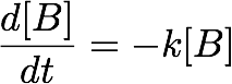
For a first order reaction with a single reactant B (e.g., a decomposition) the concentration at any given time can be determined from the following differential equation^[1]:

(3)
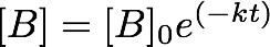
- where k is the rate constant. A solution to this equation is:
(4)
- where [B]₀ is the initial concentration. You can check that this is indeed a solution to Equation 3 by differentiating Equation 4 with respect to time. Plotting the change in concentration with respect to time will not yield a straight line, rather it will result in an exponential decay. In order to make this a linear function, we take natural logs (ln) of both sides:
(5)
- This then gives us an equation that looks awfully like a "y = mx + C" graph! Plotting ln[B] against time will yield a graph of gradient "-k" and intercept of ln[B]₀.

Revisiting the Arrhenius relationship (Equation 2), we now have a method for determining k at a number of temperatures.

Download the file "Arrhenius-1.csv" from Blackboard. This contains a sample data set from a reaction in which k has already been determined. The data show k at a range of temperatures for a given reaction.

Plot a graph of k vs T; this will require deciding which is the dependent and independent variable.
- Is this a linear relationship? Can a trendline/linear regression analysis yield results for the activation energy (E_a in Equ. 2)?
Decide if you need to take natural logarithms of the data to yield a "y = mx + C" data, and on which data it should be performed (k or T?).
- If so, take the appropriate logarithms using the Excel functions, and plot a graph of the resultant data.
- Analyse all data to report a value for E_a and the pre-exponential factor A, including units for each.

BlackBoard 'Quirk' - On this occasion you need to enter your answer in standard form, e.g. 6.02E23 if entering Avogardo's number, and for units you need report everything as a power; for example if entering ms^-1 (m/s), you need to enter as "m s^-1".

↑ This is not the full rate law, a more general term can be found in Atkins

Iterative solutions: Solver

Many chemical processes will have multiple components, and simply plotting a graph and/or taking logarithms will be insufficient to yield results. An example of this is in the analysis of fluorescent lifetime decays. Fluorescence is a phenomenon with which you will be familiar, having seen "blacklight" tubes causing clothing and accessories to glow.

Fluorescence can be measured to have a lifetime of up to ~10ns; the method used to do so is called flash photolysis, where a bright flash is used to create a large number of excited state molecules very quickly. These excited molecules then start to decay with very similar kinetics to that described in the rate-law above. The exception is that we observe the decay as emission of light, and fewer excited molecules means lower light intensity.

The difference is that there is frequently more than a single pathway by which the fluorescence is emitted, meaning that the decay curve is frequently a convolution of multiple exponential decays. A simple analysis such as that detailed in the previous section will not reveal the full amount of data possible from this curve. In order to analyse these more complex data sets, we must use an iterative solution.

Introduction to iterations

Put simply, an iterative solution is one where a 'guess' is fed into the equation and run through to find a solution; this solution is then fed back into the equation to generate a second solution, which is then fed back through the equation and so on. Ideally the solutions should converge on a single value, and this is then reported to be the 'general' solution for the problem. Excel uses the built in application 'Solver' to process iterative solutions. Its method of operation is as follows:

Generate a 'trial curve' from a possible equation
Compare the trial curve to the data set (generate an R² value)
Use the R² value to generate new starting conditions for a refined curve
Continue the comparison to minimise R².

You will use this tool to solve a flash photolysis data set which is known to have "bi-exponential decay".

Flash Photolysis data

Flash photolysis is a measure of fluorescence intensity with respect to time. The time scales are usually on the order of picoseconds, while the measure of intensity is usually the number of photon counts. For this reason, it is sometimes known as Time Correlated Single Photon Counting, or TCSPC. In a bi-exponential plot such as this, there are three key features as shown in Figure 11:

The BLUE curve is the flash, or pump, signal. It is a very brief flash from the light source, and will always show up in the signal
The GREEN curve is the exponential decay signal from a short fluorescence lifetime
The RED curve is the exponential decay signal from a longer fluorescence lifetime

The equation which governs a biexponential fluorescence lifetime (i.e., two components) is as follows:

The pre-exponential factors A₁ and A₂ govern the contribution of each exponential decay to the overall signal (so A₁+A₂ = 1 ; this will help with your analysis), while k_r₁ and k_r₂ are the respective radiative rate constants for each lifetime. The radiative rate constant for each component relate to the natural lifetime as follows:

This natural lifetime may be thought of as 'the average amount of time a molecule will remain in its excited state before it decays'

Data analysis - building a trial function

Download the data file "Flash-photolysis.csv" from the Blackboard folder and open in Excel. Select one of the five data sets to analyse first. You may find it easiest to paste this data set into its own worksheet rather than having all the data sets in the same area.

Plot a graph of the data (plotting Time, t, and Intensity, "I(data)") to see its profile. You should recognise its main features from Figure 11 above; particularly the 'rise' in intensity in the first few picoseconds as a result of the 'flash'.
An exponential decay should also be apparent after the peak intensity, in line with what was explained earlier.

The first thing to do will be to build a trial function using the biexponential decay equation:

In the cells (remember to label them!) deposit trial values for A₁, k₁, A₂ and k₂. Remember also that A₁+A₂=1 ; you may wish to define a dependence here.
Alongside your data set (e.g., if your data is in columns A and B, use column C), build your trial function
- If your data starts with t=0 in cell A5, in cell C5 build your trial function by entering the appropriate formula, drawing on your experienced gained from the techniques explored above.
- You may need to use the Excel help to find the syntax for the 'exponential' function.
- Remember to use brackets to group terms together, and do not forget the "$" operator to 'fix' the cells in which you have your trial values.
Once you are happy with the first cell, apply this to all the rest of the cells in column C; we shall call this trial curve "I(fit)":
- Either click-and-drag the bottom right corner of the first cell, or you can 'double-click' the bottom right corner - this will fill column C down to the end of the data set.
Having generated your trial function, plot it on the same graph as your data and compare the two.
- You may wish to read MATU on how this should look; search for "residuals" in the index

It is unlikely at this stage that you will have matched the curve exactly. If you 'tweak' your trial values for A₁, k₁, A₂ and k₂ (you can exclude A₂ if you defined a dependence on A₁ as it will dynamically adjust), you should see on the plot your trial function altering as you alter these values. You could alter these values manually until you can "see" a good fit, but why spend the time when we have a computer to do the work for us(!)? This is where we want to use the Solver program built into Excel.

Data analysis - installing Solver

The Solver tool may not already be installed on the computer you are using; to check (under Office 2010, most campus PCs will use this version), click "Data" and see if Solver is present under 'data analysis' in the 'Ribbon'. If not, follow the instructions at this website to install and configure Solver:

Microsoft Excel Help

Return to the "Data" ribbon and see if Solver has appeared (usually in the top right of the screen).

Data analysis - using Solver

Before we can use Solver, there are a few other things we need to do:

Ultimately in this exercise we are performing a 'least squares' analysis so, we need to find the 'squares'
- Alongside your I(fit) trial function, find the "square of the difference" between I(fit) and I(data)
- Fill the rest of this column with the "squares of the difference"
You now need to decide where the actual 'data' starts; because the data "ramps up" at the start there will of course be a huge difference between your data and your trial function in this section. If this section is included in your least-squares analysis it will lead to spurious results.
Once you have decided the region in which your data lies (somewhere after the peak), find the sum of all the squares in this region.
- You might find it convenient to do this summation in a cell near your initial trial values.

You now need to invoke Solver. This program will aim to alter any given cell, the "objective", to a maximum, a minimum, or a predefined value by changing any other cells you choose and which are linked to that "objective cell". As you are doing a least-squares analysis, we will need to minimise the sum (which you have just calculated) of all the squares . As this is dependent on the trial values A₁, k₁, A₂ and k₂, you can select these cells as "objects to be altered" in order to achieve the minimisation of the "objective cell"

Open Solver (Excel -> Tools -> Solver)
Set the objective cell as your 'sum of squares' cell
Set it to "Minimise"
Select the cells to alter.
- You should by now have defined the dependence between A₁ and A₂, meaning only three cells need be selected; A₁, k₁ and k₂
Click 'Solve'

You should now see your trial function alter and fit as best to the data as Solver can manage.

There is however rarely a single immediate solution to such problems, and Solver may not necessarily have found the correct solution, rather it may have found something called a "local minimum", rather than the "global minimum" required (see this article for more information).

To try and find if this is a local or a global minimum, try altering one of your trial parameters and running Solver again as above to see if the same values are returned as before.

Another option to try is to "restrict" your squares to a particular area of the data. As was shown in Figure 11, at either end of the decay curve, one or other of the exponential components will dominate the signal. You can use this to your advantage as follows:

Perform a 'sum of squares' on the region of interest -- you will need to identify where the transition between the two exponentials lies by looking at your plot of the data
Instruct Solver to minimise this 'restricted squares' value by altering EITHER A₁ and k₁ OR A₂ and k₂ -- but not both. This should give you a good fit to one end of the graph
Having found a fit to one end of the graph by solving for A₁ and k₁, you can now go back to solve the complete 'sum of squares' as before, but only by varying k₂ (remembering that A₁ and A₂ are linked).

Make a note of the values for A₁, k₁, A₂ and k₂, and determine the natural lifetime of each of these components.

Conduct a similar analysis for the remaining four data sets, and report your findings on the Blackboard submission.

Submission of Results

You should submit your results using Blackboard. There are two parts to the submission; the first is to enter the results of your analysis into a Blackboard Assessment. There is no time limit for this assessment; you can revisit it to continue filling it out. You can only press Finish once - if you want to revisit your answers, press Save All and close the window.

The second part of the assessment is to upload the analysis that you did - this is 'showing your working'. It should be clear in each workbook exactly how you found your answers. Ideally you should submit only one Excel workbook (or similar) containing all your work, rather than lots of individual workbooks.

The answers you give must be supported by an appropriate analysis - Answers submitted to Blackboard without support from a complete data analysis will not be awarded credit.

Final points

In this workshop material we have covered a great deal of material, and you will find all of these techniques useful to you during your course of study in Chemistry at Imperial College. While some of the techniques may not be immediately applicable in your lab classes, it is good to be aware of them, and you will find it useful to refer back to keep this page as a reference for when you come to analyse your data.

In using Solver, you will have obtained experience in using a large number of advanced Excel functions; while you may not immediately use Solver again in first year, you will certainly use the Excel experience you have gained in analysing your data.

Excel is not the only program available for data analysis; as mentioned in lectures there is a mathematical software called MatLab which has the capability of automating many of the more laborious tasks of data analysis and you may find it interesting to explore this possibility in your private study time. You can obtain a copy of MatLab for your personal use free of charge under the College site license; visit the Software Shop to find out information on this service. A MatLab primer has been written to accompany this course which you may find helpful to work though should you wish to have a go.

Go to Introduction | Go to Workshops | Go to MatLab primer

[1] This is not the full rate law, a more general term can be found in Atkins

[1]