MatLab

Matlab is an interactive and intuitive dynamic program environment based on C, Fortran and Java. A dynamic programming environment removes the need to compile your code, instead your script is parsed to a back end that does all that work for you. Matlab is well supported and the answer to almost any question can be found on Google, it is often best to Google your question before consulting the Matlab in-built help function.

Matlab finds many applications in chemistry, it can link directly to experimental apparatus and analyse results on the fly. It also allows users to completely automate data analysis leaving them more time to do more meaningful activities. It does however require care and consideration as automating a process can lead to hidden errors. For that reason all programmers will tell you the first thing you need to write code is a piece of paper. Plan what you are going to do before you start writing your program.

Theoretical work and data analysis is about thinking not just pressing buttons.

Starting Matlab

On opening Matlab you are presented with a window divided into 4 sections:

Command Window: this is where you enter commands and execute scripts, it is the workhorse of Matlab
Workspace: this lists all variables and data currently loaded in your Matlab session (normally stored in RAM or swap)
Command History: this lists every command you have ever entered in Matlab in chronological order
Current Folder: a graphical means of navigating around your computer

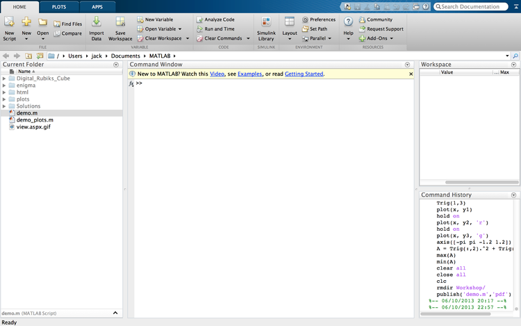
The first thing we need to do is make a folder for this workshop, Matlab has most of the standard unix commands in its libraries, in the command window type:

>> mkdir Workshop

you will see a folder called Workshop has appeared in the Current Folder pane to move into that folder type:

>> cd Workshop

cd is the unix command for change directory to move backwards you would type cd .. which in this case would take you back to the folder you started in. Now that we are in our folder we can do some operations.

Simple Operations

First lets use Matlab like a calculator

>> 1+2

you should see that Matlab has given the answer 3, next try

>> 7-2

hopefully Matlab gave you an answer of 5. Matlab obeys parenthesis in the same way as we do try

>> (7-2)*(9-4)/(3+2)

this should give you 5. As well as these simple operations Matlab has vast libraries of functions and constants, if you type

>> pi

Matlab should display 3.1416, don't worry $π$ is stored to more decimals places than that, the output is just truncated. We can also find sin $(π)$ note that Matlab uses angles in radians not degrees, to input angles in degrees use sind(x).

>> sin(pi)

As you can see Matlab does not get this right, it gives some small but non-zero value, this is due to the algorithm Matlab uses to determine sine, for most purposes this value is small enough to be considered 0. Matlab moves beyond most calculators and allows us to define variables, in fact as an imperative language variables are the core of all Matlab programming. Lets define

>> x = pi

now on typing x Matlab will return 3.1416, Matlab stands for matrix laboratory and so most things in Matlab are handled as vectors (lists of numbers) or matrices (tables of numbers) if you type

>> x = [1 pi]

you will see that you have defined x as a row vector, x has 2 values 1 and $π$ . We can also define x to be all the integers from 1 to 10

>> x = 1:10

the : tells Matlab to go from 1 to 10 in increments of 1, you will see Matlab spits out all the integers from 1 to 10. We can change the increment and the bounds, lets go from $- π$ to $π$ in increments of 0.01. In this case we don't really want Matlab to spit out all the numbers so we suppress the output using a ;. Suppressing the output not only makes your code look neater it also speeds it up - as printing information takes time.

>> x = -pi:0.01:pi;

You have now created a vector from $- π$ to $π$ , we can see how many values that has by using the size function.

>> size(x)

Matlab should tell you the size is 1 629 this means the data has one row and 629 columns. We can now make a vector $y = \sin (x)$

>> y = sin(x);

Lets take a look at the data in a plot

>> plot(x,y)

This will give you a plot of the sine wave, before closing the plot type

>> xlabel('x')
>> ylabel('Sin(x)')
>> title('Sine Wave')

then look at your plot again, and you'll see we've added some labels to it.

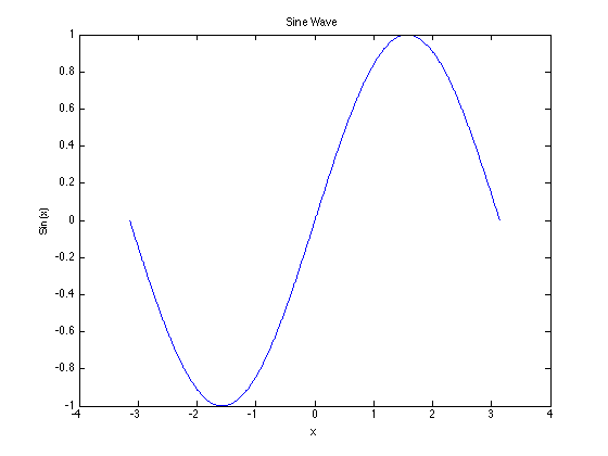
Now close your plot and lets make a table of values, firstly to make out table neat we want the data to be in column vectors to do this we need to transpose the vector x.

>> x = transpose(x);
>> size(x)

you should now see that the size of x is 629 1 so a column vector of 1 column and 629 rows. Lets make a table with $\sin (x), \cos (x)$ and $t a n (x)$ .

>> Trig = [x sin(x) cos(x) tan(x)];

The square brackets tell Matlab we want to make a matrix (or table) with columns x,sin(x),cos(x) and tan(x). If you run

>> size(Trig)

you should now see that this is a table with 629 rows and 4 columns. Lets check that everything is ok we know that $\sin^{2} (x) + \cos^{2} (x) = 1$ . Here we need to careful that we act on each element in turn and not on the data as a matrix. To do element-wise operations we use a . before the operation so for example A*B is matrix A times matrix B (matrix multiplication) whereas A.*B returns a new matrix where each element of A has been multiplied by its counterpart in B. If in doubt always use . before the operations *,/ and ^. So lets check our identity

>> A = Trig(:,2).^2 + Trig(:,3).^2;

Note here that Trig(:,2) refers to all the rows in column 2, Trig(:,:) would be everything in the table Trigand Trig(2,:) would be everything in row 2. Also that we use ^ for power with ., there is never a . needed for + or -. So lets see if the identity is returned by checking the maximum and minimum value of A.

>> max(A)
>> min(A)

Matlab should return 1 for both cases and the identity is returned. Finally lets plot all these curves on the same axis, to this we will need to use hold to tell Matlab we want to add a new line to the plot

>> plot(Trig(:,1), Trig(:,2))
>> hold on

lets make the next line a dotted red one

>> plot(Trig(:,1), Trig(:,3), '.r')
>> hold on

and the final line a dashed green line

>> plot(Trig(:,1), Trig(:,4), '--g')
>> xlabel('x')
>> ylabel('y')
>> title('Trigonometric Functions')

but there is a problem if you look at the plot because $\tan (x) \to \infty$ as $\cos (x) \to 0$ it obliterates all the other lines, we can rectify this by constraining the axes using the axis([xmin xmas ymin ymax]) command, so before closing your plot type

>> axis([-pi pi -1.2 1.2])

now if you look at your plot everything should be in slightly better order. Finally lets add a legend to the plot, though hopefully it is not necessary in this case.

>> legend('Sin(x)', 'Cos(x)', 'Tan(x)')

Now your plot is finished!

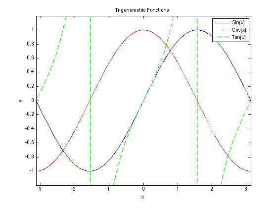
If you look in the Workspace pane you'll see it has been filled with variables, we should clear those before continuing

>> clear all

you should see everything disappear, now lets close the plots

>> close all

and finally lets make the command line a bit neater

>> clc

These operations wiped the memory and cleared the command line, this should be done at the start of every Matlab session and every Matlab script. If it is not done you run a huge risk of errors creeping in. So far we have only used the command window which is not much good, really we want to write scripts that we can save and run over again or run without needing any user input. To do this we open a new Matlab script click on the New Script icon in the top left hand corner and the editor will open up.

Scripting with Matlab

Whatever we type in a Matlab script is executed in the command window, lets plot the Sine wave with our first script to demonstrate this


close all
clear all
clc 

x=-pi:0.01:pi;
y=sin(x);

plot(x,y)
xlabel('x')
ylabel('Sin(x)')
title('Sine Wave')

To run this script click on the green run triangle, Matlab will prompt you to save it as something and then it will produce a Sine curve. One of the most commonly used tools in programming is a loop a loop tells the computer to repeat a task X many times so

for X=1:1000

do something

end

will carry out the same operation 1000 times, this is important if you want to calculate some properties and store them in a table. The best way to explain for loops is through summation lets try to calculate $\sum_{n = 1}^{1000} n$ ok so this is a pretty easy sum we know the value must be 500500. In Matlab we would do this by a loop, lets write a new script to do this.

close all
clear all
clc

for ii=1:1000
   S = S + ii;
end

Save and run this script, Matlab will give you an error as we haven't defined S! A great strength of Matlab is that it has clear error messages, if you get them read them carefully ... they will often lead you straight to the problem so we should correct the script to

close all
clear all
clc

S = 0; %sum starts at 0


for ii=1:1000
   S = S + ii;
end

If you run this and type S into the Command Window Matlab should return 500500. Note that every for must have an end, you can nest loops but each nested loop must be ended. You'll notice that anything after the % sign is in green, this is a comment in Matlab. A comment is a note to yourself or someone else that is not passed to the computer, comments are very important they should be used to explain in human terms what you are doing. That way you or anyone else can pick up your code in the future and see what you were doing. Lets say we wanted to calculate $\sum_{n = 1}^{100} n - \frac{n^{3}}{3!} + \frac{n^{5}}{5!} - \frac{n^{7}}{7!}$ and also we wanted to know the value of the sum at every $n$ , to do this we need to build a matrix of values from our loop, either start a new script or continue on after your sum script.

close all
clear all
clc 


S = 0;

for ii = 1:1000
  Value(ii,1) = ii;
  S = S + ii - (ii.^3)/factorial(3) + (ii.^5)/factorial(5) - (ii.^7)/factorial(7);
  Value(ii,2) = S;
end

If we then plot Value we should see how the sum is behaving in the Command Window plot the summation.

>> plot(Value(:,1), Value(:,2))

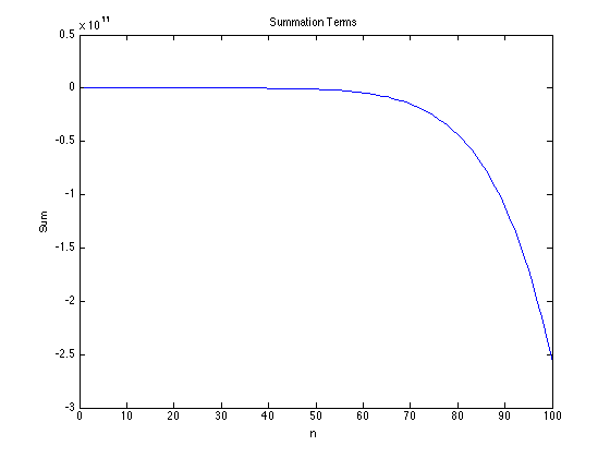
So far we have been using = without much thought, it is important to know that in any C based language = means assign. So we are saying that x is assigned as 4. If you think about it in the summation examples S = S + ii for example is only true when = is being used in the mathematical sense if ii is 0. To test if 2 things are equal in Matlab we use == this tells Matlab to do a true or false check.

It is probably easiest to see in an example lets write a simple program that tells us if a number is odd or even. To do this we will use the mod function, the mod function returns 1 there is a remainder from a division and 0 if there is not. So mod(4,2)=0 whereas mod(4,3)=1. Our program needs to:

Take a value in from the user
Check that it is an integer (only integers can be odd or even)
Check if it is odd or even
Tell the user

So how can we check an integer well any integer divided by 1 will leave no remainder, any real non-integer divided by 1 will give a remainder so mod(x,1)=0 for all integers and 1 for all non-integers. If the number is even mod(x,2)=0 and if is odd mod(x,2)=1. Lets give it a go. Open a new script and type

clear all
close all
clc

x = input('Enter an integer:');

if mod(x,1) == 0
   if mod(x,2) == 0
      disp('The number is even')
   else 
      disp('The number is odd')
   end
else 
   error('Please enter an integer')
end

Save and run your program, try entering an odd integer, an even integer and a non-integer. Note there are 2 if statements and so 2 end statements in the script. Hopefully this quick tutorial will give you enough knowledge to complete the tasks, if you have any problems remember we are all here to help.

Polynomials

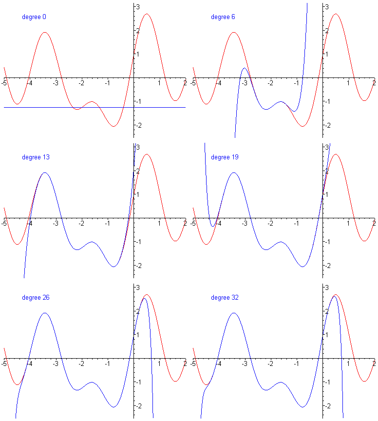
Polynomials are functions of the form $y = \sum_{n = 0}^{N} a_{n} x^{n}$ , in this workshop you will use a polynomial fit. Polynomials are of great importance in theoretical work as they can approximate any continuous differentiable function in a given range, this known as Taylor's theorem. Below is an example of a polynomial fit around $x = - 2$ for the function $y = e^{\cos (x)} \sin (x) + \cos (2 x) s i n (π x)$ , as the degree (highest power) of the polynomial gets larger the polynomial approaches the function when the degree is $\infty$ then the polynomial exactly maps the function.

Disclaimer

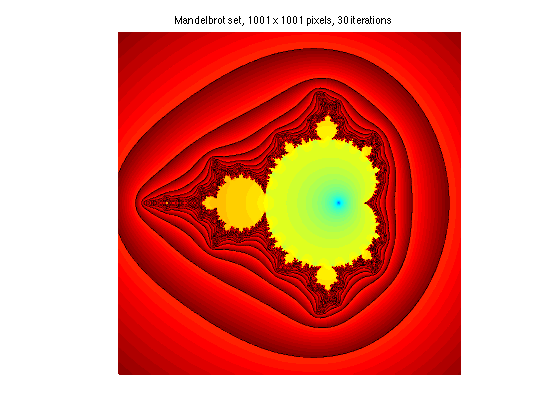
We have barely scraped the surface of Matlab's capabilities here, it can plot complex things like the Mandelbrot set

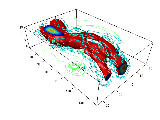
or 3D functions

and polar functions.

It can even be used to paint with mathematics!

The code for these plots is available here: [1]