Visualizing High Model Orbitals
Visualizing High Model Orbitals
Aim
When using ONIOM we are often interested in the effect of an environment on the model compound. For this reason it is often useful to visualize the orbitals of the high model region after a calculation. When trying to do this in Gaussview, however, it is found that the orbitals displayed are those of the low model. This is the reason why it was necessary to construct orbitals using guess=input in the ONIOM(CASSCF:AM1) examples. This tutorial explains how to access the orbitals after a calculation has been run, for example if we wish to localize orbitals to ensure the correct active space has been chosen in the previous example. In the case of QM:MM calculations it is possible to skip the punch orbitals step as there is only one set of orbitals on the checkpoint file; just get the model geometry and read the guess from the checkpoint file directly (I think newer versions of Gaussian actually die now if you try to do this - Lee).
System
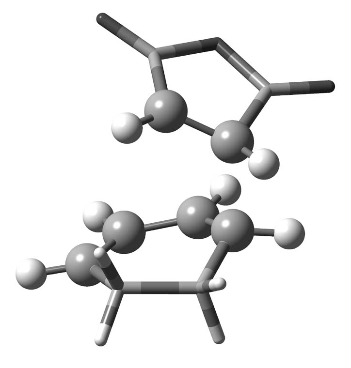
In this tutorial we examine the spurious transition state in the diels-alder cycloaddition between maleic anhydride and cyclohexadiene. We extract the high model orbitals and localize them to ensure that the correct active space has been chosen. This allows us to check that the choice of active space is not the cause of disagreement with the high real calculation, which indicates a symmetric transition state.

Method
Punch Orbitals
The first task is to obtain the orbitals if the high model in a format that can be read back in by Gaussian. This can be achieved using the punch=MO keyword but, in order to punch the high model orbitals we need to use a nonstandard route.
First we use testrt to obtain the standard route:
 -----------------------------------------------------------------
 #p oniom(casscf(6,6)/sto-3g:hf/sto-3g) guess=read nosymm punch=MO
 -----------------------------------------------------------------
 1/38=1,52=2/1;
 2/12=2,15=1,17=6,18=5,40=1/2;
 1/38=1,52=2,53=3172/20;
 3/6=3,11=9,16=1,25=1,30=1,116=-2/1,2,3;
 4/5=1,17=6,18=6/1;
 5/5=2,38=6/2;
 6/7=2,8=2,9=2,10=2,28=1/1;
 1/52=2,53=2032/20;
 3/6=3,16=1,25=1,32=1,116=101/1,2,3;
 4/5=1,17=6,18=6/1,5;
 5/5=2,17=1000000,38=6/10;
 6/7=2,8=2,9=2,10=2,28=1/1;
* 1/52=2,53=1022/20;
* 3/6=3,11=9,16=1,25=1,30=1,116=-2/1,2,3;
* 4/5=1,17=6,18=6/1;
* 5/5=2,38=6/2;
* 6/7=2,8=2,9=2,10=2,28=1/1;
* 1/52=2,53=3014/20;
 99/5=1,9=1,10=32/99;
The asterisked lines can be removed as they correspond to the low real system and adjust the last line to read 99/10=32/99. We can now construct the input file to punch out the high-model orbitals. Remember to add cp fort.7 $WORK/$FLD/$FLNM.orbs to your jobscript file after the gaussian execution line as this file will contain the punched orbitals.
%nprocshared=2
%mem=2000MB
%chk=/work/lmt09/PHD_Y2/MALA_CYHEX/ONIOM/macyhexdiene_S0_SPpunch_oniom_cas66_sto3g_hf_sto3g
# nonstd
1/38=1,52=2/1;
2/12=2,15=1,17=6,18=5,40=1/2;
1/38=1,52=2,53=3172/20;
3/6=3,11=9,16=1,25=1,30=1,116=-2/1,2,3;
4/5=1,17=6,18=6/1;
5/5=2,38=6/2;
6/7=2,8=2,9=2,10=2,28=1/1;
1/52=2,53=2032/20;
3/6=3,16=1,25=1,32=1,116=101/1,2,3;
4/5=1,17=6,18=6/1,5;
5/5=2,17=1000000,38=6/10;
6/7=2,8=2,9=2,10=2,28=1/1;
99/10=32/99;

#p oniom(casscf(6,6)/sto-3g:hf/sto-3g) guess=read nosymm punch=MO
Punch high model orbitals for localization

0 1 0 1 0 1
 H                0   -0.26330500   -1.99941700   -1.21363800 H
 C                0    0.78714900    1.41335300    0.46807900 H
 C                0    1.26328700    1.66455000   -0.88162300 H
 O                0   -1.92502500   -0.01205900    2.50907200 L
 C                0    2.10729300    0.78800800   -1.50119200 H
 H                0    0.93300900    2.55923500   -1.39147400 H
 C                0    2.36471400   -0.53645200    0.68140600 L H 9   0.0000
 C                0   -0.44009500   -1.08924500    0.83298900 H
 C                0    1.08572800    0.18779800    1.13172100 H
 C                0   -0.78359900   -1.36617800   -0.51617700 H
 C                0    2.60670600   -0.49404400   -0.84831600 L H 5   0.0000
 O                0   -2.42068300    0.13236600    0.27717100 L
 C                0   -1.63821400   -0.28747100    1.36303200 L H 8   0.0000
 H                0    2.12198000   -1.34178900   -1.33290700 L
 O                0   -2.47630400   -0.31974200   -1.96661200 L
 H                0    3.67299000   -0.60346100   -1.04369100 L
 C                0   -1.93186300   -0.50956600   -0.89422500 L H 10   0.0000
 H                0    0.08918800    2.11204200    0.91605600 H
 H                0   -0.01783200   -1.85015200    1.47955400 H
 H                0    0.96794500    0.21509600    2.21057000 H
 H                0    2.35971100   -1.57164700    1.01714300 L
 H                0    3.19920800   -0.04865300    1.18673800 L
 H                0    2.42869300    0.97055600   -2.52117800 H
Obtain Geometry
Now we have the orbitals for the high model in the .orbs file, however, if we wish to visualize these with gaussview we need to have them in a Gaussian output and so we need the geometry of the high model system. This can be done by taking the geometry output by the optimization and using the onlyinputfiles option.
%nprocshared=1
%mem=800MB
%chk=/work/lmt09/PHD_Y2/MALA_CYHEX/ONIOM/macyhexdiene_S0_SPinput_oniom_cas66_sto3g_hf_sto3g
#p oniom(casscf(6,6)/sto-3g:hf/sto-3g)=onlyinputfiles nosymm

Input files

0 1 0 1 0 1
 H                0   -0.26330500   -1.99941700   -1.21363800 H
 C                0    0.78714900    1.41335300    0.46807900 H
 C                0    1.26328700    1.66455000   -0.88162300 H
 O                0   -1.92502500   -0.01205900    2.50907200 L
 C                0    2.10729300    0.78800800   -1.50119200 H
 H                0    0.93300900    2.55923500   -1.39147400 H
 C                0    2.36471400   -0.53645200    0.68140600 L H 9   0.0000
 C                0   -0.44009500   -1.08924500    0.83298900 H
 C                0    1.08572800    0.18779800    1.13172100 H
 C                0   -0.78359900   -1.36617800   -0.51617700 H
 C                0    2.60670600   -0.49404400   -0.84831600 L H 5   0.0000
 O                0   -2.42068300    0.13236600    0.27717100 L
 C                0   -1.63821400   -0.28747100    1.36303200 L H 8   0.0000
 H                0    2.12198000   -1.34178900   -1.33290700 L
 O                0   -2.47630400   -0.31974200   -1.96661200 L
 H                0    3.67299000   -0.60346100   -1.04369100 L
 C                0   -1.93186300   -0.50956600   -0.89422500 L H 10   0.0000
 H                0    0.08918800    2.11204200    0.91605600 H
 H                0   -0.01783200   -1.85015200    1.47955400 H
 H                0    0.96794500    0.21509600    2.21057000 H
 H                0    2.35971100   -1.57164700    1.01714300 L
 H                0    3.19920800   -0.04865300    1.18673800 L
 H                0    2.42869300    0.97055600   -2.52117800 H
Localizing Orbitals
The final part is to combine these two calculations to produce a Gaussian output with the orbitals on the high model. The first step is to copy and paste the high model input file from the onlyinputfiles output. Remember this is a single layer calculation so ensure that no ONIOM keywords are present. Once this is done add guess=cards to the route (note that in the example below the IOps have been removed as they are not necessary) and copy the .orbs file to the bottom of the input file. If localized orbitals are desired the vaarious keywords can be added here. This results in the following input:
Media:Male_loc.gjf
We can now visualize the results which reveal a p-orbital on each carbon of the high model region, showing the correct active space has bee chosen. Media:Male_loc.log
