User talk:Sw4512cmp

Show that the lowest possible energy for the Ising model is E = -DNJ.

It is given $E$ = $$\begin{gathered} -\frac{1}{2}J\sum _i^N\sum _{j \\ \in \\ \mathrm{n}\mathrm{e}\mathrm{i}\mathrm{g}\mathrm{h}\mathrm{b}\mathrm{o}\mathrm{u}\mathrm{r}\mathrm{s}\left(i\right)}{s}_i{s}_j \end{gathered}$$, where $s_i,s_j\in \{-1,1\}$ and $J$ is a constant.

To achieve the most negative expression for $E$ requires all pairs of multiples $s_i\times s_j=1$ within the double sum. Since the multiplication is done upon all neighbouring pairs, one can infer for a single connected lattice:

$$\begin{gathered} s_i=s_j \\ \mathrm{\forall } \\ i,j \end{gathered}$$

The outer summation sums over N elements, for each of the N elements, the inner summation sums all its neighbours, the number of which is a function of the dimensionality D. In a Cartesian sense, the inclusion of an additional orthogonal direction will increase the number of neighbours by 2. Hence:

$$\begin{gathered} \sum _i^N\sum _{j \\ \in \\ \mathrm{n}\mathrm{e}\mathrm{i}\mathrm{g}\mathrm{h}\mathrm{b}\mathrm{o}\mathrm{u}\mathrm{r}\mathrm{s}\left(i\right)}{s}_i{s}_j \end{gathered}$$ = $$\begin{gathered} \sum _i^N\sum _{j \\ \in \\ \mathrm{n}\mathrm{e}\mathrm{i}\mathrm{g}\mathrm{h}\mathrm{b}\mathrm{o}\mathrm{u}\mathrm{r}\mathrm{s}\left(i\right)}1 \end{gathered}$$ = $N\times (2\times D)$

Overall:

$E$ = $$\begin{gathered} -\frac{1}{2}J\sum _i^N\sum _{j \\ \in \\ \mathrm{n}\mathrm{e}\mathrm{i}\mathrm{g}\mathrm{h}\mathrm{b}\mathrm{o}\mathrm{u}\mathrm{r}\mathrm{s}\left(i\right)}{s}_i{s}_j=-DNJ \end{gathered}$$

The condition $$\begin{gathered} s_i=s_j \\ \mathrm{\forall } \\ i,j \end{gathered}$$ can be satisfied by $s_i=s_j=1or{s}_i=s_j=-1$, therefore without an external magnetic field, there are two microstates with the lowest possible energy. Hence the multiplicity of the system is 2.

Using the Boltzmann's entropy equation: $S=k_{\mathrm{B}}\ln W$ where W is the total number of microstates and $k_{\mathrm{B}}$ the Boltzmann constant. The entropy $S=k_{\mathrm{B}}\ln 2$

NJ: Good, include the numerical value as well

Imagine that the system is in the lowest energy configuration. To move to a different state, one of the spins must spontaneously change direction ("flip"). What is the change in energy if this happens ($$\begin{gathered} D=3, \\ N=1000 \end{gathered}$$)? How much entropy does the system gain by doing so?

When an arbitrary spin is flipped from the lowest energy configuration, all the favourable interactions between it and its neighbours (of which it has 6 when D = 3) are turned into unfavourable interactions. As six favourable interactions disappear, and also six unfavourable interactions are created, the change in energy is $+12J$, given each neighbouring spin interaction contributes to one energy unit.

In the first excited state, there will be one spin that is anti-parallel to all the other spins. The number of microstates that can achieve this is $2N$.

Therefore, $\mathrm{\Delta }S=S_{excited}-S_{ground}=k_B(ln(W_{excited})-ln(W_{ground}))=k_B(ln(2N)-ln(2))=k_{B}ln(N)$

Numerically, $S=9.53\times 10^{-23}kJ{K}^{-1}$

I think that's the entropy of the new state, not the increase, but correct otherwise.

Magnetisation Calculations

$M=\sum _i{s}_i$. The 1D configuration on the right has magnetisation of +1. While the 2D one is also +1.

For T = 0 K, the system should assume the lowest energy configuration possible, so the magnetisation could equally take a value of +N or -N without an applied external magnetic field regardless of the system dimension nor the total number of spins. (D=3,N = 1000)

Figure: Illustration of an Ising lattice in one (N=5), two (N=5x5), and three (N=5x5x5) dimensions. Red cells indicate the "up" spin", and blue cells indicate the "down" spin.

Output of energy() and magnetisation() functions

Calling the ILcheck.py function gives the following output:

Output from ILcheck.py

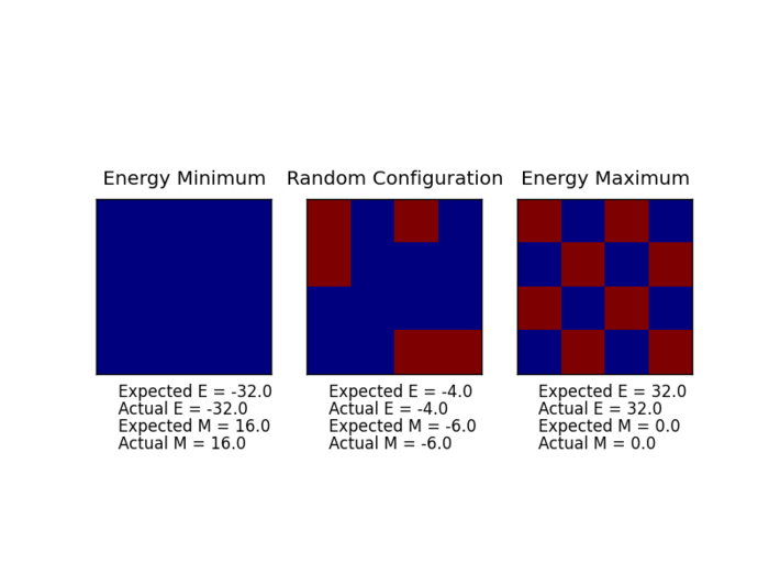
Suggestingthe energy() and magnetisation() functions are correct.

The complete code will be presented as a whole class in a later section.

The need for significance sampling

For a system of 100 spins, there are in total of $2^{100}$ configurations. With the given processing speed of $1\times 10^9{s}^{-1}$ it will take $1.3\times 10^{21}$ seconds to sample all the configurations to work out averages, or equivalently over $4\times 10^{13}$ years to analyses all these configurations sequentially.

IsingLattice class

The completed IsingLattice.py class is presented as below:

import numpy as np

class IsingLattice:
    E = 0.0
    E2 = 0.0
    M = 0.0
    M2 = 0.0
    n_cycles = 0

    
    #constants definitions:
    k_b = 1.0;
    Dimension = 2
    J = 1.0
    step_ignore = 30000

    def __init__(self, n_rows, n_cols):
        self.n_rows = n_rows
        self.n_cols = n_cols
        self.lattice = np.random.choice([-1,1], size=(n_rows, n_cols))
        
        
    #helper function defined for ease of setting lattice config	for debugging
    def set(self, i, j, spin):
        self.lattice[i][j] = spin;
        return;
        

    #the less efficient way to calculate energy via element-wise sum
    #i.e. E = sum(current element * sum(all its four neigbours))
    #its speed has been measured by using ILtimetrial.py script
    def energySlow(self):
        "Return the total energy of the current lattice configuration."
        energy = 0;
        for i in range(self.n_rows):
            for j in range(self.n_cols):
                energy += self.lattice[i][j] * (self.lattice[(i-1)%self.n_rows][j] + self.lattice[(i+1)%self.n_rows][j] + \
        self.lattice[i][(j-1)%self.n_cols] + self.lattice[i][(j+1)%self.n_cols]);
        return -0.5 * self.J * energy;
        

    #Faster implementation to calculate energy
    #Each spin in the lattice defined by a matrix M is element-wise multiplied by the element-wise sum of its right neighbour R and 
    #its bottom neighbour B. The cumulative sum of the resulting matrix is produced, i.e. E = sum(M.*(R+B))
    #its speed characterised by using ILtimetrial.py script
    def energy(self):
        energy = np.sum(np.multiply(self.lattice, (np.roll(self.lattice, 1, axis = 0) + np.roll(self.lattice, 1, axis = 1))));
        #no double counting so the factor of 0.5 is not needed.
        return float(-self.J * energy);
        
    #Return the total magnetisation of the current lattice configuration.
    def magnetisation(self):
        magnetisation = np.sum(self.lattice);
        #return float to ensure float division is always performed when magnetisation is involved
        return float(magnetisation);


    def montecarlostep(self, T):
        E0 = self.energy();
        random_i = np.random.choice(range(0, self.n_rows));
        random_j = np.random.choice(range(0, self.n_cols));
        self.lattice[random_i][random_j] *= -1;
        E1 = self.energy();
        deltaE = E1 - E0;

        #favourable energy, accept state
        if (deltaE < 0):
            E0 = E1;
        
        else:
            random_number = np.random.random();
            if (np.exp(-(deltaE/(self.k_b * T))) >= random_number):
                #accept new state 
                E0 = E1;
            else:
                #revert back to old config
                self.lattice[random_i][random_j] *= -1;
        
        energy, magnetisation = E0, self.magnetisation();
        
        #updates, one should account for far more steps after equilibrium than the steps ignored pre-equilibrium, 
        #thus by evaluating the following if statement first should save a little bit of execution time
        if self.step_ignore <= 0 :
            #print("here")
            self.E += energy;
            self.E2 += (energy**2);
            self.M += magnetisation;
            self.M2 += (magnetisation**2);
            self.n_cycles += 1;
        else:
            self.step_ignore -= 1;
            
        return energy, magnetisation;
        

    def statistics(self):
        #if @self.step_ignore has not reached zero, it is assumed system
        #has not reached equilibrium, so results are not meaningful,
        # so -1 are returned in that case.
        if (self.step_ignore <= 0):
            aveE = self.E/self.n_cycles;
            aveE2 = self.E2/self.n_cycles;
            aveM = self.M / self.n_cycles;
            aveM2 = self.M2 / self.n_cycles;
            return aveE, aveE2, aveM, aveM2, self.n_cycles;
        return -1, -1, -1, -1, -1;

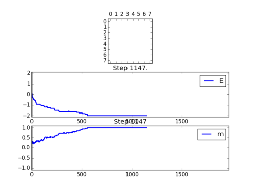
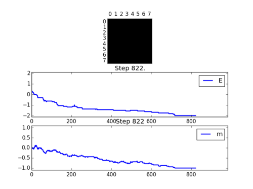
If $T<T_C$, do you expect a spontaneous magnetisation (i.e. do you expect $⟨M⟩\ne 0$)? When the state of the simulation appears to stop changing (when you have reached an equilibrium state), use the controls to export the output to PNG and attach this to your report

The simulations below are performed at 0.5K, which is far below (approx. 2.5 K below from later finding) the critical temperature for such a system size and thus one would expect the state of equilibrium to be one of the two lowest energy configurations. The outputs below shows these to be the case and indeed both states can be approached depending on the initial random configurations.

NJ:Careful, this isn't in Kelvin. It's reduced temperature units

In general, when $T<T_C$, spontaneous magnetisation would occur as the level of thermally induced fluctuation is not enough to disrupt the overall magnetic dipole.

For the Positve spin, the text output of the ILanim.py file looks as below: (The quantities are not divided by the total number of spins in the system)

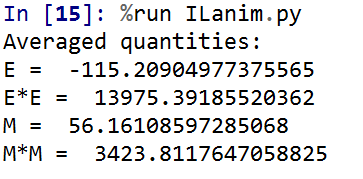
For the final state, energy should equal to -128J while magnetisation should equal to 64 in this case. But as the averaging takes into account of steps prior to equilibrium, the output values are smaller than the ones stated.

Performance comparison

For the calculation where the energy is calculated by the energySlow() function in the IsingLattice class, time taken to perform 2000 Monte Carlo steps on a 25x25 lattice is:

$t_{2000}$ = 6.98 ± 0.0207 s

While using the faster energy() function yields the following:

$t_{2000}$ = 0.327 ± 0.000681 s

As the numpy.sum() function was already known to the author, the magnetisation function has not been changed.

The standard error is calculated after 1000 repeats. The code was executed using a Intel i5-2540M 2.60 GHz CPU and the Python 3.4.1 |Anaconda 2.1.0 environment.

How many cycles are typically needed for the system to go from its random starting position to the equilibrium state? .

Using the standard code given (8x8 lattice 1.0 K) the following graph is generated:

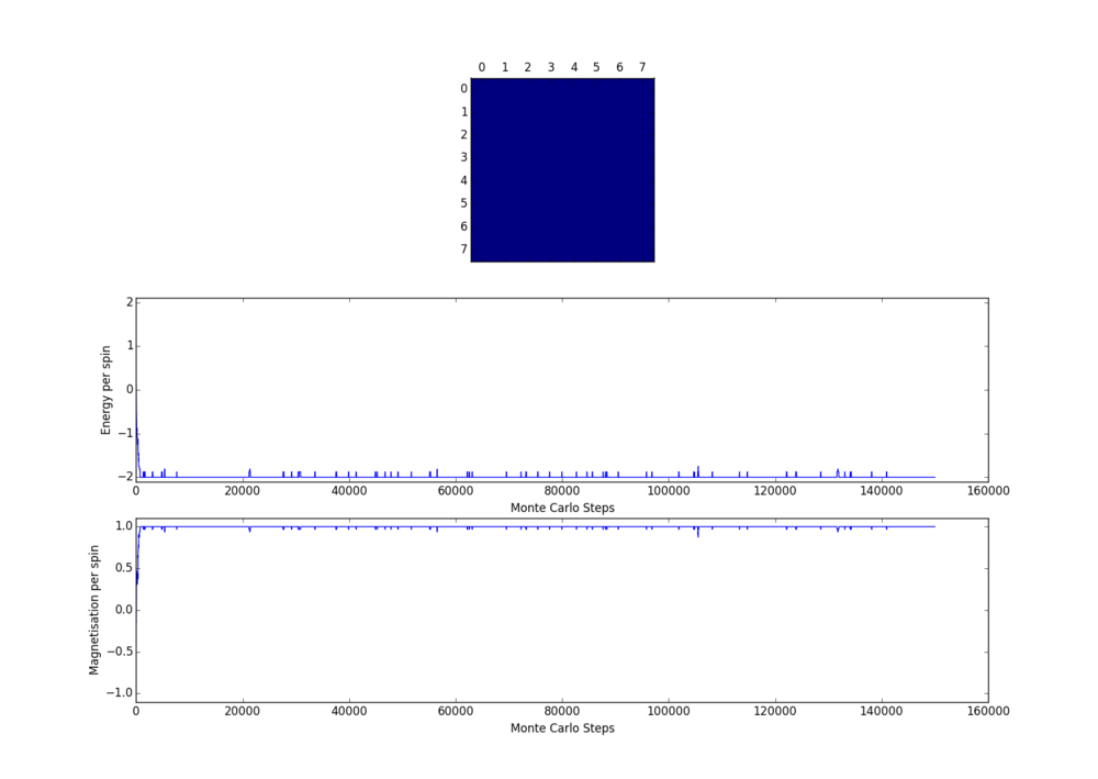
One can see the lowest energy state is reached and maintained after less than 10000 steps. A few repeats shows similar outcome.

However, it is thought that with increased lattice size and increased temperature, equilibrium state will be more difficult to reach. Some test on 32x32 lattice were done at 0.5 K and 5.0 K - the two temperature extremes at which further simulations were carried out. The following two graphs show the behaviour for 32x32 lattice at 0.5 K.

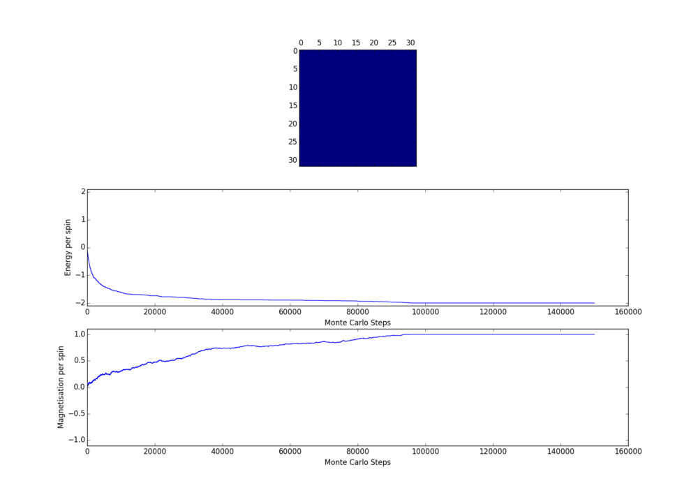
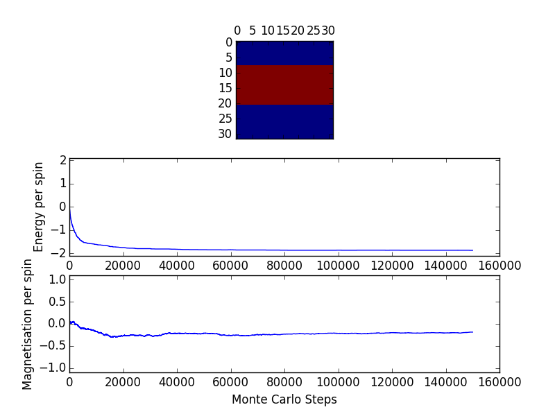
One can see sometimes the lowest energy state is not the equilibrium state. But in both cases, after about 30000 steps the energy values have more or less become flat. It is slightly surprising to see that in fact for high temperature of 5.0 K (see the 2 figures below) equilibrium is reached almost instantaneously.

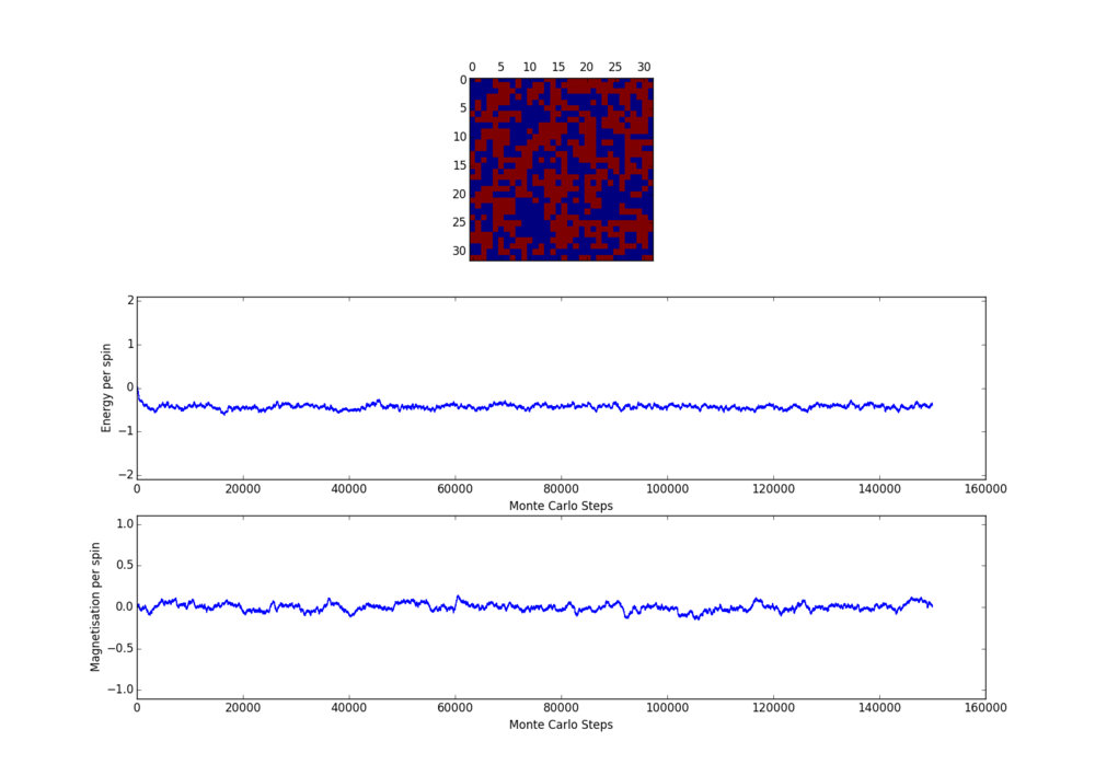
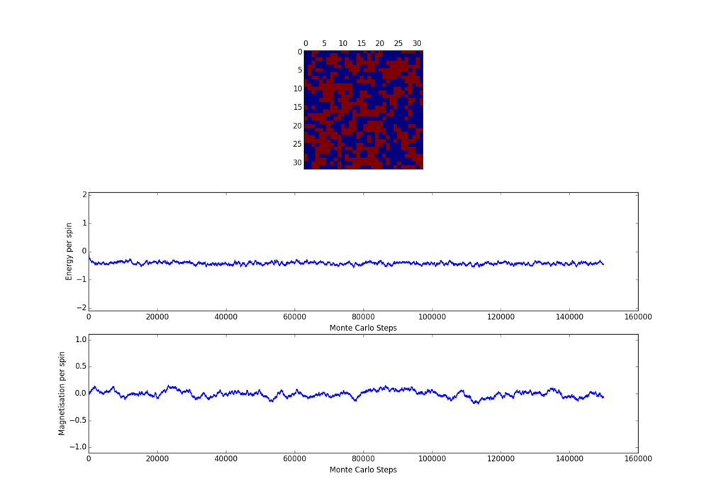
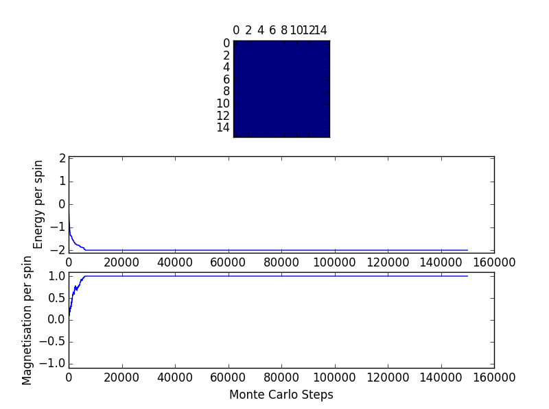
The number of steps to ignore is chosen to be 30000 steps. This is because after 30000 steps, energy has become stable (reached a plateau ) for configurations that takes the longest to reach equilibrium (low temperature, large lattices).

A back of the envelope calculation using execution times from the previous section suggests if the overall simulation runs for 300000 steps ,i.e. the first 10% of the simulation is ignored (which the author intend to do), it should take around 1 minute to run the 32x32 lattice at a given temperature. This means to run simulations from 0.5 to 5.0 K in small increments (0.1 K) will take less than a hour to complete. Such time is acceptable. However one can see by ignoring 30000 steps cannot guarantee the magnetisation will reach an equilibrium. To do so will require ignoring more than 90000 steps. This will increase the overall simulation time by 3-fold and this increment in time is not worth-while as the primary goal of the simulation involves finding heat capacity, which relies on good energy estimation only.

Experiment on low and high temperature 16x16 lattice (below) also demonstrate ignoring 30000 steps is more than enough.

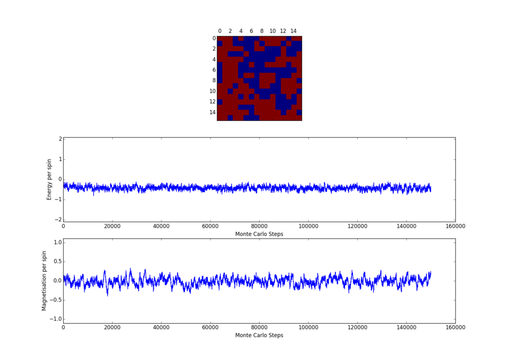
One misconception the author had was that at low temperature (approx 0.5 K) the lattice should necessarily reach the lowest energy state. This seems to be not the case from the above simulations for large lattices and this suggests it depends also on the starting configuration. Further investigation at the extreme case, when the starting lattice configuration is at the highest energy possible state, shows the energy minimum was not reached even after several million steps for 8x8 lattices.

NJ: Yes, it's always possible to get into a sort of pathological state in which you keep going round in circles, so to speak. It's unlucky, though!

The highest lattice configuration is achieved using the "set" function in the IsingLattice class in conjunction with the following code snippet):

il = IsingLattice(n_rows, n_cols);

pre_spin = 1;

for i in range(n_rows):
    cur_spin = pre_spin;
    for j in range(n_cols):
        il.set(i, j, cur_spin);
        cur_spin *= -1;
    pre_spin *= -1;

To check if the energy minimum state has been reached, the lattice is element-wise multiplied with a matrix of ones and the absolute value of the cumulative sum should equal to the dimension of the matrix:

''np.absolute(np.sum(np.multiply(np.ones(shape = (n_rows, n_cols)), il.lattice))) == n_rows * n_cols''

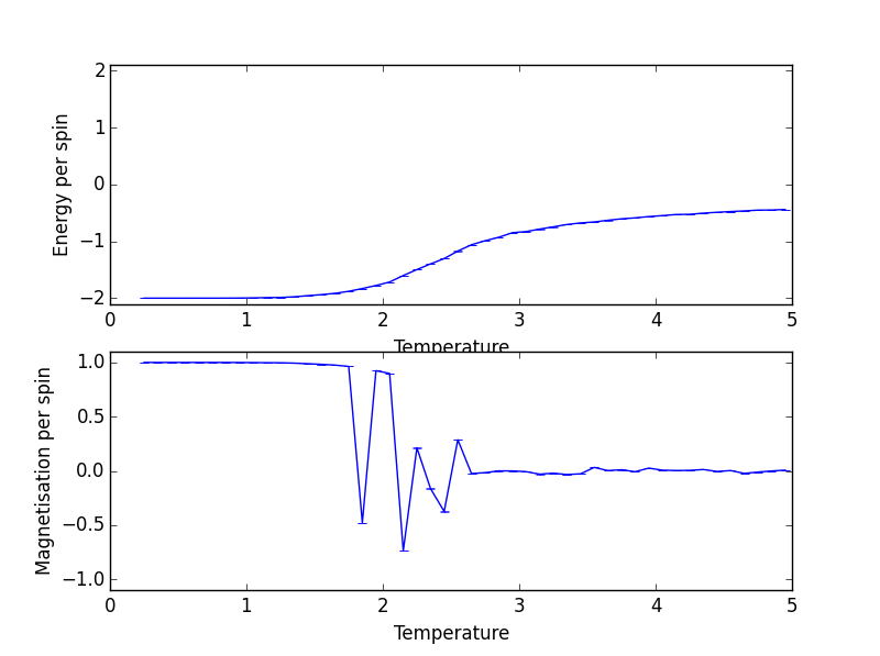
Use ILtemperaturerange.py to plot the average energy and magnetisation for each temperature, with error bars, for an 8x8 lattice

The temperature is sampled starting from 0.25 K upto and including 4.95 K in 0.1 K intervals. And an overall $3\times 10^5$ steps are run. As $3\times 10^4$ steps are considered pre-equilibrium, the reminder 90% of the simulation is used to extract averages.

from IsingLattice import *
from matplotlib import pylab as pl
import numpy as np

n_rows = 2
n_cols = 2
il = IsingLattice(n_rows, n_cols)
runtime = 300000
cycles = 0;
spins = n_rows*n_cols
times = range(runtime)

#temperature intervals
temps = np.arange(0.25, 5, 0.1)

energies = []
magnetisations = []
energysq = []
magnetisationsq = []
for t in temps:
    for i in times:
        energy, magnetisation = il.montecarlostep(t)
    aveE, aveE2, aveM, aveM2, cycles = il.statistics()
    energies.append(aveE)
    energysq.append(aveE2)
    magnetisations.append(aveM)
    magnetisationsq.append(aveM2)
    
    #reset the IL object for the next cycle
    il = IsingLattice(n_rows, n_cols)
    il.lattice = np.ones((n_rows, n_cols))    

#calculating the standard errors from the obtained arrays from above
ene_error = np.sqrt((energysq - np.square(energies))/cycles)
mag_error = np.sqrt((magnetisationsq - np.square(magnetisations))/cycles)

#Graph plotting
fig = pl.figure()
enerax = fig.add_subplot(2,1,1)
enerax.set_ylabel("Energy per spin")
enerax.set_xlabel("Temperature")
enerax.set_ylim([-2.1, 2.1])
magax = fig.add_subplot(2,1,2)
magax.set_ylabel("Magnetisation per spin")
magax.set_xlabel("Temperature")
magax.set_ylim([-1.1, 1.1])
enerax.errorbar(temps, np.array(energies)/spins, yerr = ene_error/spins)
magax.errorbar(temps, np.array(magnetisations)/spins, yerr = mag_error/spins)
pl.show()

#data saving in "lattice size_sw4512.dat" format
final_data = np.column_stack((temps, energies, energysq, magnetisations, magnetisationsq))
np.savetxt(str(n_cols) + "x" + str(n_rows) + "_sw4512.dat", final_data)

Output from ILtemperaturerange.py for a lattice size of 8x8 is shown below:

Repeat the final task of the previous section for the following lattice sizes: 2x2, 4x4, 8x8, 16x16, 32x32. How big a lattice do you think is big enough to capture the long range fluctuations?

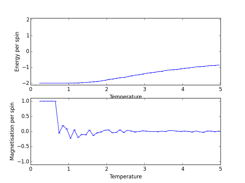
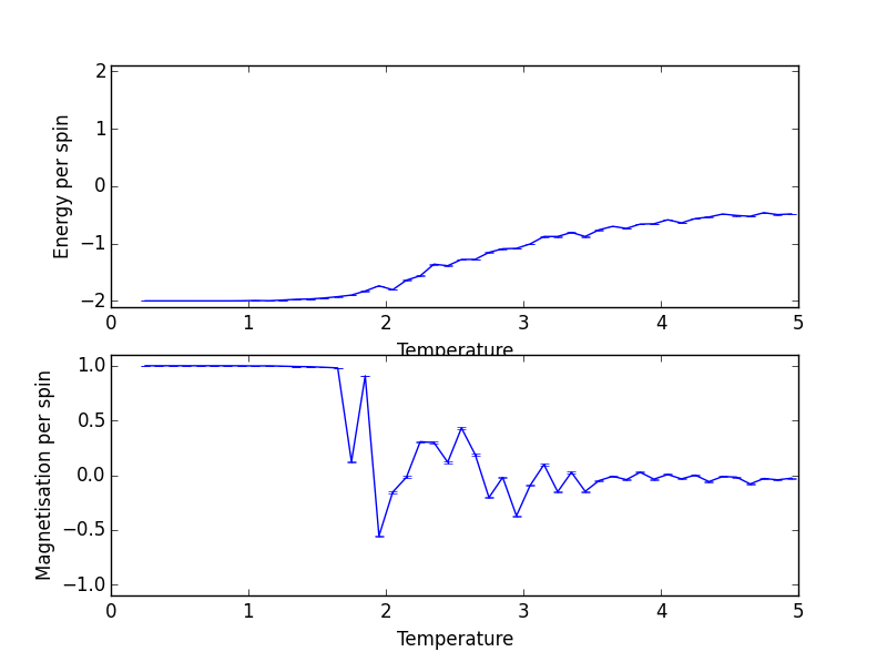
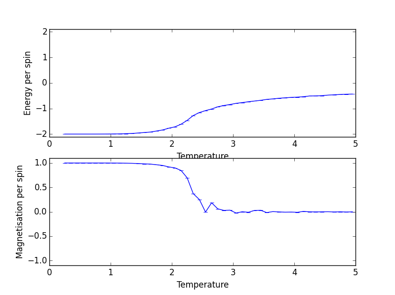
By changing the "n_rows" and "n_cols" attributes in the code segment in the above section, 2x2, 4x4, 16x16 and 32x32 lattices are simulated and the plots with error bars are presented below:

Energy and Magnetisation per Spin against Temperature for 2x2 Lattice Size

---

Energy and Magnetisation per Spin against Temperature for 4x4 Lattice Size

---

Energy and Magnetisation per Spin against Temperature for 8x8 Lattice Size

---

Energy and Magnetisation per Spin against Temperature for 16x16 Lattice Size

---

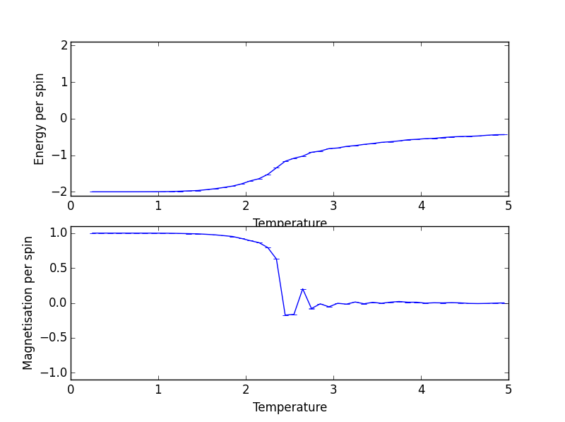
Energy and Magnetisation per Spin against Temperature for 32x32 Lattice Size

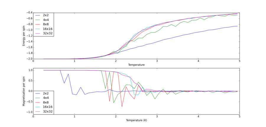
The graphs are plotted onto the same set of axis and is shown below: By looking at the magnetisation, one can see for lattice of all sizes spontaneous magnetisation disappears with increasing temperature. Looking at the energy graph, one can see the trajectory between 8x8, 16x16 and 32x32 hardly differ and suggests lattice size of 8x8 is already large enough to capture long range fluctuations.

The code used to achieve the above is:

from IsingLattice import *
from matplotlib import pylab as pl
import numpy as np

fig = pl.figure()
enerax = fig.add_subplot(2,1,1)
enerax.set_ylabel("Energy per spin")
enerax.set_xlabel("Temperature (K)")
magax = fig.add_subplot(2,1,2)
magax.set_ylabel("Magnetisation per spin")
magax.set_xlabel("Temperature (K)")
magax.set_ylim([-1.1, 1.1])

for i in range(5):
    size = 2**(i + 1);
    spins = size**2;
    matrix = np.loadtxt(str(size)+"x"+str(size)+"_sw4512.dat");
    temps, energies, energysq, magnetisations, magnetisationsq = matrix[:,0], matrix[:,1], matrix[:,2], matrix[:,3], matrix[:,4];
    
    enerax.plot(temps, np.array(energies)/spins, label= str(size)+"x"+str(size))
    enerax.legend(loc=2, borderaxespad=0.0);
    magax.plot(temps, np.array(magnetisations)/spins, label= str(size)+"x"+str(size))
    magax.legend(loc=3, borderaxespad=0.0);
pl.show()

Write a Python script to make a plot showing the heat capacity versus temperature for each of your lattice sizes from the previous section

As $C=\frac{\mathrm{V}\mathrm{a}\mathrm{r}[E]}{k_B{T}^2}$, where $$\begin{gathered} Var[E]= \\ <E^2>-<E{>}^2 \end{gathered}$$, the following code was written to obtain the heat capacity and temperature plots for the various lattice sizes with the obtained "energies" and "energysq" values:

from IsingLattice import *
from matplotlib import pylab as pl
import numpy as np

k_b = 1;

fig = pl.figure()
heatcap = fig.add_subplot(1,1,1)
heatcap.set_ylabel("Heat Capacity")
heatcap.set_xlabel("Temperature (K)")

for i in range(5):
    size = 2**(i + 1);
    spins = size**2;
    matrix = np.loadtxt(str(size)+"x"+str(size)+"_sw4512.dat");
    temps, energies, energysq = matrix[:,0], matrix[:,1], matrix[:,2];
    var = energysq - np.square(energies)
    heatcap.plot(temps, np.divide(var,(np.square(temps)*k_b)), label= str(size)+"x"+str(size))
    heatcap.legend(loc=2, borderaxespad=0.0);
pl.show()
    

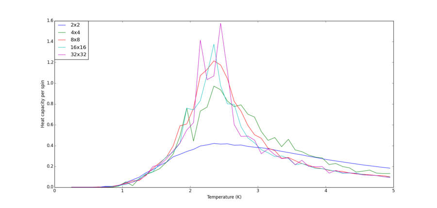
The outcome is shown below:

NJ: Good! Just a note, you can always use the "".format() method as well to add data to strings.

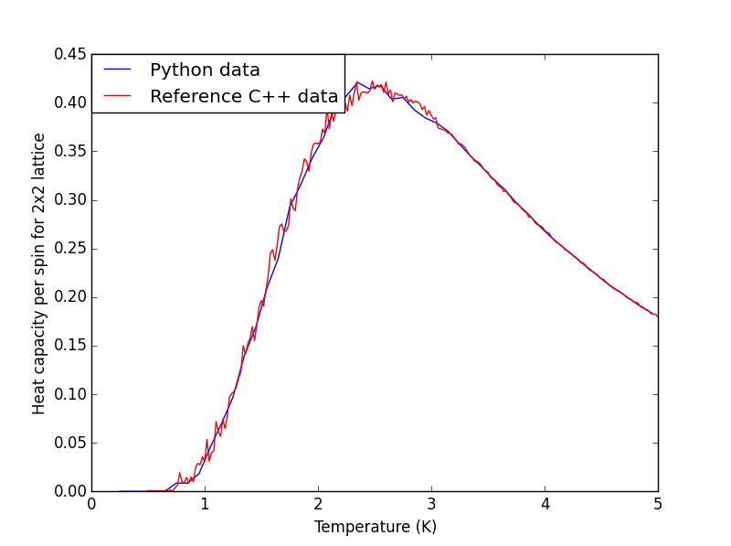
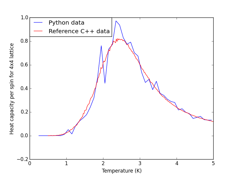
Plot the C++ data against your data

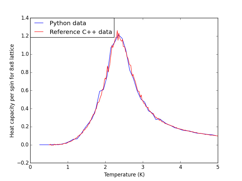
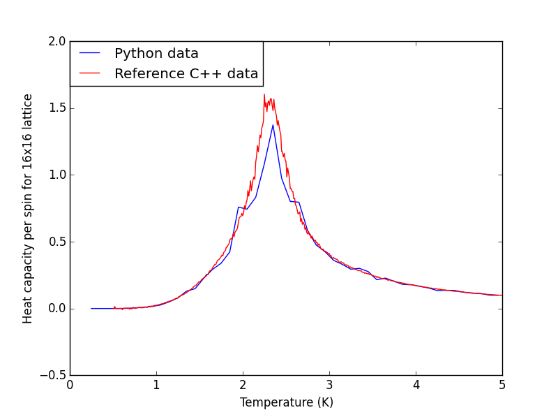
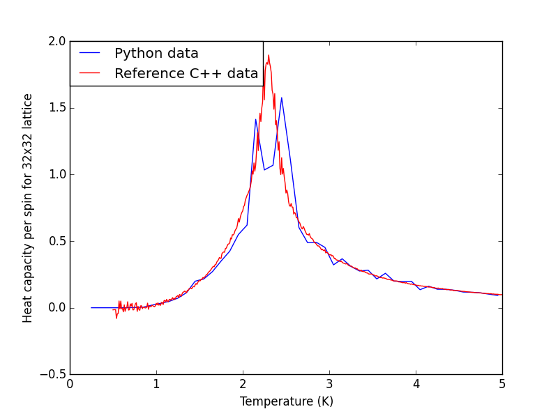
The plots for all the lattice sizes show the two sets of data fits quite well, although for 32x32 the python data seems slightly lower than the C++ data, which could suggest more steps needs to be ignored prior to equilibrium.

Heat Capacity Against Temperature Plots for Different Lattice Sizes

The code used is shown below:

from IsingLattice import *
from matplotlib import pylab as pl
import numpy as np

k_b = 1;

for i in range(5):
    size = 2**(i + 1);
    spins = size**2;
    fig = pl.figure()
    heatcap = fig.add_subplot(1,1,1)
    heatcap.set_ylabel("Heat capacity per spin for " + str(size) + "x" +str(size) + " lattice")
    heatcap.set_xlabel("Temperature (K)")

    matrix = np.loadtxt(str(size)+"x"+str(size)+"_sw4512.dat");
    temps, energies, energysq = matrix[:,0], matrix[:,1], matrix[:,2];
    var = energysq - np.square(energies)
    heatcap.plot(temps, np.divide(var,(np.square(temps)*k_b))/spins, label= "Python data")
    
    
    matrix = np.loadtxt("../C++/" + str(size)+"x"+str(size)+".dat");
    temps, heat_cap = matrix[:,0], matrix[:,5];
    heatcap.plot(temps, heat_cap, "r", label= "Reference C++ data")
    
    heatcap.legend(loc=2, borderaxespad=0.0);
    pl.show()
    

Write a script to read the data from a particular file, and plot C vs T, as well as a fitted polynomial. Try changing the degree of the polynomial to improve the fit

For this experiment, the 32x32 lattice is used. Starting with an second order polynomial, the total terms is doubled and the attempt fit is plotted against the raw C++ data. With increased polynomial terms the fitting becomes better but one can see there is hardly any change from 64 degree up to 256, suggesting convergence (512 degree polynomial seems to break the algorithm and produce a far worse fit). With some further experimentation, it is found 442 degree polynomial marks the onset of the algorithmic breakdown.

NJ: Nice figure!

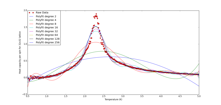
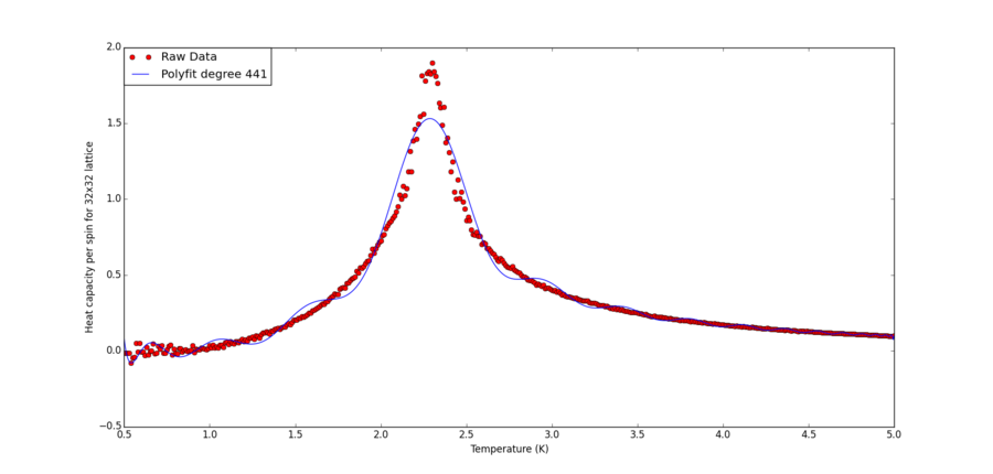
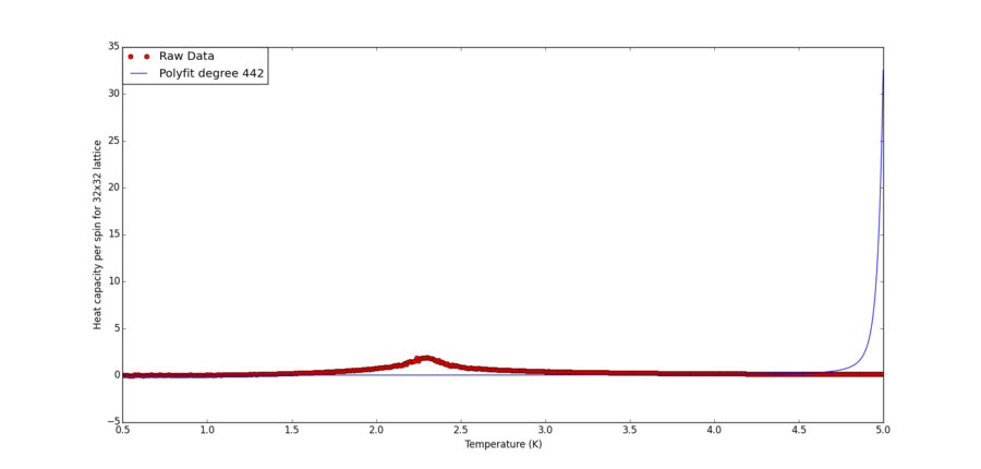
As shown, the fitting is rather poor. This means it is difficult if at all possible to obtain the full heat capacity curve in an analytically form using purely polynomial terms in T.

The code used is as shown below:

from IsingLattice import *
from matplotlib import pylab as pl
import numpy as np

k_b = 1;
size = 32;
    
fig = pl.figure()
heatcap = fig.add_subplot(1,1,1)
heatcap.set_ylabel("Heat capacity per spin for " + str(size) + "x" +str(size) + " lattice")
heatcap.set_xlabel("Temperature (K)")

matrix = np.loadtxt("../C++/" + str(size)+"x"+str(size)+".dat");
T, C = matrix[:,0], matrix[:,5];
heatcap.plot(T, C, "ro", label= "Raw Data")
degree = 1    
for i in range(8):
    degree *= 2;
    fit = np.polyfit(T, C, degree) # fit a third order polynomial
    T_min = np.min(T)
    T_max = np.max(T)
    T_range = np.linspace(T_min, T_max, 1000) #generate 1000 evenly spaced points between T_min and T_max
    fitted_C_values = np.polyval(fit, T_range) # use the fit object to generate the corresponding values of C    
    heatcap.plot(T_range, fitted_C_values, label= "Polyfit degree " + str(degree))
    heatcap.legend(loc=2, borderaxespad=0.0);
pl.show()

Modify your script from the previous section. You should still plot the whole temperature range, but fit the polynomial only to the peak of the heat capacity

The partial fit uses the following code:

from IsingLattice import *
from matplotlib import pylab as pl
import numpy as np

k_b = 1;
size = 32;


    
fig = pl.figure()
heatcap = fig.add_subplot(1,1,1)
heatcap.set_ylabel("Heat capacity per spin for " + str(size) + "x" +str(size) + " lattice")
heatcap.set_xlabel("Temperature (K)")
matrix = np.loadtxt("../C++/" + str(size)+"x"+str(size)+".dat");
T, C = matrix[:,0], matrix[:,5];
heatcap.plot(T, C, "ro", label= "Raw Data")
degree = 1   

for i in range(8):
    degree += 1;
    
    T_min = 2.0
    T_max = 2.5

    selection = np.logical_and(T > T_min, T < T_max);
    peak_T_values = T[selection]
    peak_C_values = C[selection]
    fit = np.polyfit(peak_T_values, peak_C_values, degree) # fit a third order polynomial
    
    T_range = np.linspace(T_min, T_max, 1000) #generate 1000 evenly spaced points between T_min and T_max
    fitted_C_values = np.polyval(fit, T_range) # use the fit object to generate the corresponding values of C    
    heatcap.plot(T_range, fitted_C_values, label= "Polyfit degree " + str(degree))
    heatcap.legend(loc=2, borderaxespad=0.0);
pl.show()
    

Essentially, the only difference from previous code segment is to change "T_min " and "T_max" from "np.min(T)" and "np.max(T)" to values closer to the peak region, which is roughly between 1.7 K and 2.7 K (with slight deviations between lattice of difference sizes).

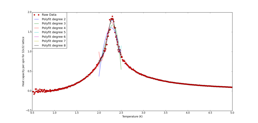
From the zoomed in plot, one can see degree 7 and degree 8 polynomial has more or less converged and both are very good fit of the raw data. Additionally no features of overfitting can be seen, The convergence suggests the algorithm has reached its optimal fit.

Find the temperature at which the maximum in C occurs for each datafile that you were given. Determine $T_{C,\mathrm{\infty }}$. Discuss briefly what you think the major sources of error are in your estimate.

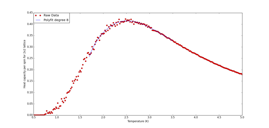
Using the code below, the heat capacity fitting is plotted for each lattice size files. Essentially, the segment differs from the one from previous section by removing the for loop that tries different degrees of polyfits. Changes to the "size" variable and "T_min" and "T_max" are made for lattice of different sizes. Polynomial of order 8 is chosen because it gives good fit to the lattice of largest size, which has the sharpest peak. Thus it should be sufficient to fit smaller lattice with milder peaks which can be represented via polynomials more easily.

from IsingLattice import *
from matplotlib import pylab as pl
import numpy as np

k_b = 1;
size = 2;


fig = pl.figure()
heatcap = fig.add_subplot(1,1,1)
heatcap.set_ylabel("Heat capacity per spin for " + str(size) + "x" +str(size) + " lattice")
heatcap.set_xlabel("Temperature (K)")

matrix = np.loadtxt("../C++/" + str(size)+"x"+str(size)+".dat");
T, C = matrix[:,0], matrix[:,5];
heatcap.plot(T, C, "ro", label= "Raw Data")
degree = 8   

T_min = 2.0
T_max = 2.5
    
selection = np.logical_and(T > T_min, T < T_max);
peak_T_values = T[selection]
peak_C_values = C[selection]

fit = np.polyfit(peak_T_values, peak_C_values, degree) # fit a third order polynomial
T_range = np.linspace(T_min, T_max, 1000) #generate 1000 evenly spaced points between T_min and T_max
fitted_C_values = np.polyval(fit, T_range) # use the fit object to generate the corresponding values of C   
 
heatcap.plot(T_range, fitted_C_values, label= "Polyfit degree " + str(degree))
heatcap.legend(loc=2, borderaxespad=0.0);
pl.show()

Heat Capacity Against Temperature Plots for Different Lattice Sizes

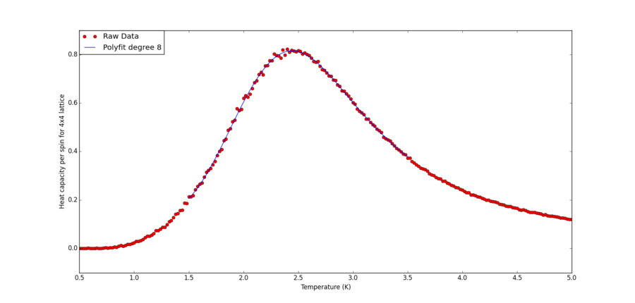
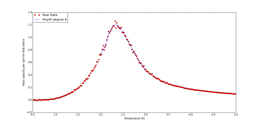
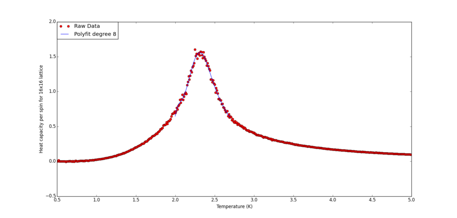
For each plot, the statement:

T_range[fitted_C_values == np.max(fitted_C_values)] gives the maximum T value for a given lattice

It is given $T_{C,L}=\frac{A}{L}+T_{C,\mathrm{\infty }}$, where $T_{C,L}$ is the Curie temperature of an $L\times L$lattice, $T_{C,\mathrm{\infty }}$ is the Curie temperature of an infinite lattice. A plot of maximum T against 1/L allows determination of $T_{C,\mathrm{\infty }}$ as the y-intercept.

The following code produces the plot below:

from pylab import *

degree = 1
h=np.loadtxt("T_infi.txt")
L = 1/h[:,0]
Tc = h[:,1]

#fitting
fit = np.polyfit(L, Tc, degree) 
equation = "T = " + str(round(fit[0],4)) + '/L' ' + ' + str(round(fit[1],4)) 
T_range = np.linspace(0, 0.6, 1000) 
fitted_C_values = np.polyval(fit, T_range) 

#plotting
xlabel('1/(Side Length) 1/L')
ylabel('Tempearture at Maximum Heat Capacity')
title('Graph to determine the Curie Temperature of Infinite 2D Ising Lattice')
plot(L, Tc,"x",label="Raw data")
plot(T_range, fitted_C_values, label= "Linear Fit: " + equation)
legend(loc=1, borderaxespad=0.0);

show()

Lattice Side Length L	Curie Temperature (K)	Fitting Range (K)
32	2.2952953	1.7-3.5
16	2.31321321	1.5-3.5
8	2.33633634	2.0-3.0
4	2.44494494	2.0-2.7
2	2.52162162	2.0-2.5

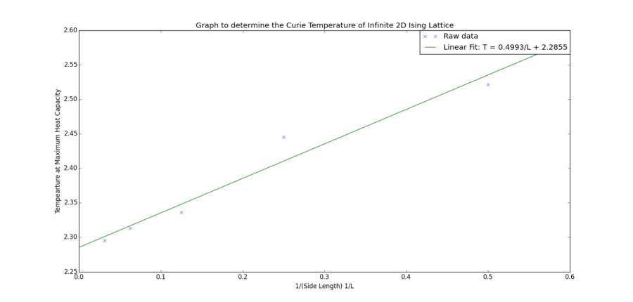Theoretical $T_{C,\mathrm{\infty }}$ can be found by solving the following condition :

$sinh(2J/k_B{T}_{C,\mathrm{\infty }})sinh(2J^{\prime }/k_B{T}_{C,\mathrm{\infty }})=1$

As in this experiment square lattices are used thus J is assumed to equal to 1, J = J' = 1 and $k_B$ is set to equal to 1.:

$sinh(2/k_B{T}_{C,\mathrm{\infty }}{)}^2=1$

$T_{C,\mathrm{\infty }}=2÷arcsinh(1)$

the value of $T_{C,\mathrm{\infty }}$ is approximately 2.2692 K.

The value extrapolated from the graph and the theoretical value differ by 0.7%.

NJ: very close, good work.

Sources of error:

The difference between the obtained value and theoretical value is in the second decimal place. The number of points sampled has a minor effect on the estimation. Typically the fitting of the peak spans over 1 K, and 1000 data points are then generated in that range. This means the difference between two neighbouring temperature points is 0.001 K, this can affect the precision of the estimate. Indeed when 1000000 points temperature points are used and a better peak can be extracted, the intercept can be reduced to 2.2822.

NJ: That's true, but do you think this is a major source of error?

It was also found that by changing the fitting range slightly, one can obtain different curie temperatures for a given lattice size. For 2x2 and 4x4 sized lattice, this change is in the second decimal point, while it is milder for larger lattices. This means for the smaller sized lattices, as the peak is not very sharp, the maxima is more ambiguous, and thus can depend more strongly on the position of individual data points, which is subjected to elements of randomness by the nature of the simulation. Therefore with allowance of computation cost, larger lattices should be used to extrapolate the trend, or one can also try smaller temperature increments during the simulation so there are more points around the peak for better statistics.

NJ: Or you could ignore the very small lattices

References

- ↑ Onsager, Lars, "Crystal Statistics. I. A Two-Dimensional Model with an Order-Disorder Transition", Phys. Rev., 1944, 65 (3-4), pp117--149 92 DOI:10.1103/PhysRev.65.117