User talk:JFU1608
JC: General comments: Most tasks completed, but some results and explanations missing from the final few tasks. Try to make your explanations clearer and more focused and use the background theory to support your answers.
Part 1: Running first simulation
-no tasks-
Part 2: Introduction to molecular dynamics simulation
Task 1
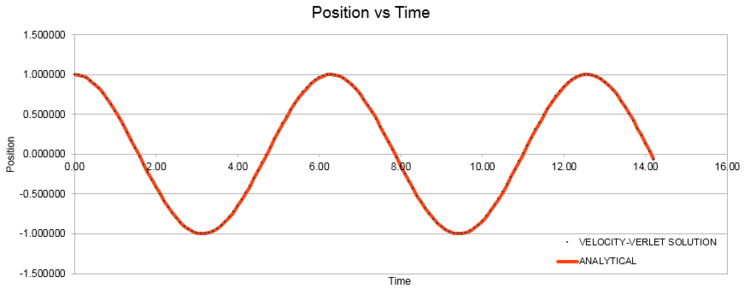
Open the file HO.xls. In it, the velocity-Verlet algorithm is used to model the behaviour of a classical harmonic oscillator. Complete the three columns "ANALYTICAL", "ERROR", and "ENERGY": "ANALYTICAL" should contain the value of the classical solution for the position at time t, "ERROR" should contain the absolute difference between "ANALYTICAL" and the velocity-Verlet solution (i.e. ERROR should always be positive -- make sure you leave the half step rows blank!), and "ENERGY" should contain the total energy of the oscillator for the velocity-Verlet solution. Remember that the position of a classical harmonic oscillator is given by (the values of , , and are worked out for you in the sheet).
ANALYTICAL: Position at time t (classical solution)
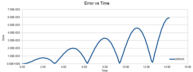
ERROR: Absolute difference between ANALYTICAL and Velocity-verlet solution
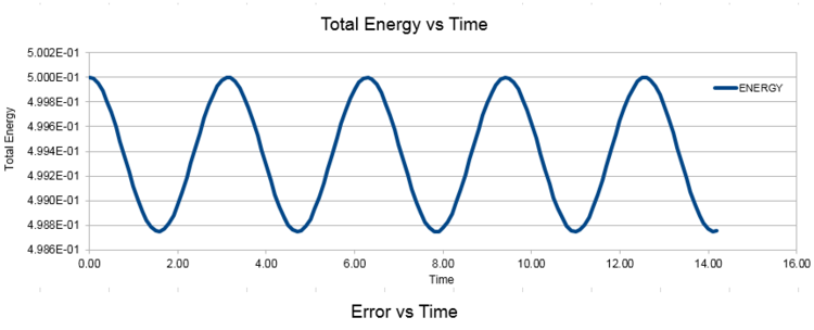
ENERGY: Total E of oscillator for velocity-verlet solution Total Energy is given by the summation of both kinetic energy: 1/2 mv2 and potential energy 1/2kx2.
Task 2
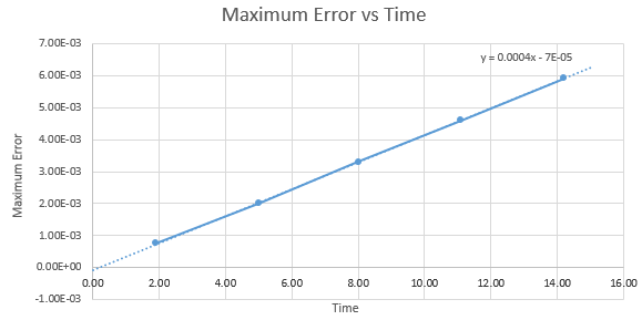
For the default timestep value, 0.1, estimate the positions of the maxima in the ERROR column as a function of time. Make a plot showing these values as a function of time, and fit an appropriate function to the data.
| Time | Maximum Error |
|---|---|
| 1.9 | 7.58E-04 |
| 5.00 | 2.00E-03 |
| 8.00 | 3.30E-03 |
| 11.10 | 4.60E-03 |
| 14.20 | 5.91E-03 |
Graph shows a linear relationship between the maximum errors of position with time, characterised by its extrapolation formula y = 0.0004x – 0.00005.
Task 3
Experiment with different values of the timestep. What sort of a timestep do you need to use to ensure that the total energy does not change by more than 1% over the course of your "simulation"? Why do you think it is important to monitor the total energy of a physical system when modelling its behaviour numerically?
Previously for timestep 0.1, the percentage change was 0.248%. By varying the timestep, we are able to deduce the corresponding percentage changes, shown in Table X. As timestep increases, the minima total energy value decreases gradually, leading to a larger percentage change in total energy. In order for total energy not to go over 1%, the timestep must not be larger than 0.2. It is important to monitor the total energy of a physical system while modelling its behaviour numerically. This is because the Law of Conservation of Energy is observed, where total energy stays constant.
| Timestep | Energy Maxima | Energy Minima | Change in Energy |
|---|---|---|---|
| 0.05 | 0.5 | 0.4997 | 0.06% |
| 0.1 | 0.5 | 0.4988 | 0.24% |
| 0.15 | 0.5 | 0.4972 | 0.56% |
| 0.2 | 0.5 | 0.4950 | 1.00% |
| 0.25 | 0.5 | 0.4922 | 1.56% |
| 0.3 | 0.5 | 0.4888 | 2.24% |
Row highlighted in bold is the simulation done from previous tasks.
JC: Good, thorough investigation of different timesteps.
Task 4
For a single Lennard-Jones interaction,  , find the separation,
 ![]() , at which the potential energy is zero. What is the force at this separation? Find the equilibrium separation,
, at which the potential energy is zero. What is the force at this separation? Find the equilibrium separation, ![]() , and work out the well depth (
, and work out the well depth (![]() ). Evaluate the integrals
). Evaluate the integrals ![]() ,
, ![]() , and
, and ![]() when
when ![]() .
.
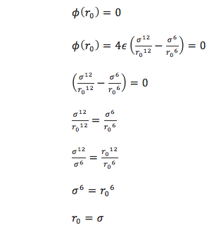
Where the potential energy is zero, separation r0 can be found:
At this separation, the force can be calculated with ![]() , where using the definition of U from equation 10 [1] produces:
, where using the definition of U from equation 10 [1] produces:
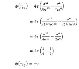
The equilibrium separation, req occurs where Fi = 0, so:
Well depth,
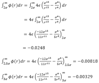
When σ=ϵ=1.0,
Task 5
Estimate the number of water molecules in 1ml of water under standard conditions. Estimate the volume of 10000 water molecules under standard conditions.
At standard conditions, there are 3.35 x 10²² water molecules in 1 mL of water. Density of water = 1 g cm-3; Volume = 1 mL = 1 cm3; Mr = 18; NA = 6.022 x 10²³
For 10000 water molecules, the calculated volume is 2.99 x 10⁻¹⁹ mL:
JC: All maths and calculations correct and nicely laid out.
Task 6
Consider an atom at position (0.5, 0.5, 0.5) in a cubic simulation box which runs from (0, 0, 0) to (1, 1, 1). In a single timestep, it moves along the vector (0.7, 0.6, 0.2) . At what point does it end up, after the periodic boundary conditions have been applied?.
Sum of (0.5, 0.5, 0.5) and (0.7, 0.6, 0.2) gives (1.2,1.1,0.7), but this assumes periodic boundary conditions not applied. If applied, number of atoms inside box always constant as one leaves, simultaneously another enters. Hence deduct (1.2,1.1,0.7) by value of 1 in the x and y coordinates since they exceed the value of 1, to give the (0.2,0.1,0.3) position.
JC: You have taken 1 away from the z coordinate as well, the final position should be (0.2, 0.1, 0.7).
Task 7
The Lennard-Jones parameters for argon are ![]() . If the LJ cutoff is
. If the LJ cutoff is ![]() , what is it in real units? What is the well depth in kJ mol-1 ? What is the reduced temperature
, what is it in real units? What is the well depth in kJ mol-1 ? What is the reduced temperature ![]() in real units?
in real units?
JC: Values are correct, but give answers to the same number of significant figures as in the question (2 in this case).
Part 3: Equilibration
Task 1
Why do you think giving atoms random starting coordinates causes problems in simulations? Hint: what happens if two atoms happen to be generated close together? If molecules are put extremely close to each other then they might overlap each other, having unfavourable repulsion interactions.
If atoms were given random starting coordinates in simulations, there is a possibility that the simulation puts 2 atoms such that they overlap one another, which is not possible in real terms. As two atoms get closer together, their potential energy increases exponentially, causing a discrepancy in the calculated values. This is avoided when the atoms are placed at lattice points.
JC: You are right that the problem is the possibility of 2 atoms being placed very close together with high repulsion between them. The high repulsion can make the simulation unstable and a smaller timestep is needed to stop it from crashing.
Task 2
Satisfy yourself that this lattice spacing corresponds to a number density of lattice points of 0.8. Consider instead a face-centred cubic lattice with a lattice point number density of 1.2. What is the side length of the cubic unit cell?
Given previously that each length of a unit cell is 1.07722,
For a fcc lattice of lattice point number density 1.2:
Task 3
Consider again the face-centred cubic lattice from the previous task. How many atoms would be created by the create_atoms command if you had defined that lattice instead?
Since the fcc lattice has 4 atoms, where each is 1000 unit cells, a total of 4000 atoms will be created.
JC: Correct.
Task 4
Using the LAMMPS manual, find the purpose of the following commands in the input script:

The first line is a mass command where 1 is the atom type, with mass of 1.0. This input script sets all atoms of atom type 1 to have a mass of 1.0.
The second line is a pair style command which computes the pairwise interactions of 2 atoms. This command is scripted such that the Lennard-Jones potential is cut off for coulomb interaction beyond distance of 3.0, hence absence of potential energy. Within distance 3.0, there will be a presence of potential energy due to the active Lennard-Jones interaction.
The third line is a pair coeff command, where the * sign in pair coeff command sets coefficients for multiple pairs of atom types. As there is no numeric value, it means all types from 1 to N. In the case used, there are only atoms of 1 type so this command sets the coefficient value to all atoms of type 1. The first 1.0 coefficient value corresponds to the distance at which potential energies, σ of 2 atoms is 0, whereas the second 1.0 coefficient is the well depth.
JC: Good, full explanations.
Task 5
The second line (starting "variable timestep...") tells LAMMPS that if it encounters the text ${timestep} on a subsequent line, it should replace it by the value given. In this case, the value ${timestep} is always replaced by 0.001. In light of this, what do you think the purpose of these lines is? Why not just write:

The first code allows the simulation to run over a fixed time with a varied amount of timesteps. Such that the larger the timestep, the lesser steps is used to run the total simulation. Similarly, more steps are used when a small timestep is set for that variation. The timestep difference between each simulation is 0.001. The second code does not allow this to happen as it only runs the simulation for a fixed timestep at 0.001.
JC: Defining the timestep using a variable means that changing the simulation's timestep involves changing only one line of the script, rather than having to manually change evry command that depends on the timestep.
Task 6
Given that we are specifying ![]() and
and ![]() , which integration algorithm are we going to use?
, which integration algorithm are we going to use?
As xi(0) and vi(0) is given, the Velocity-Verlet algorithm should be used.
Task 7
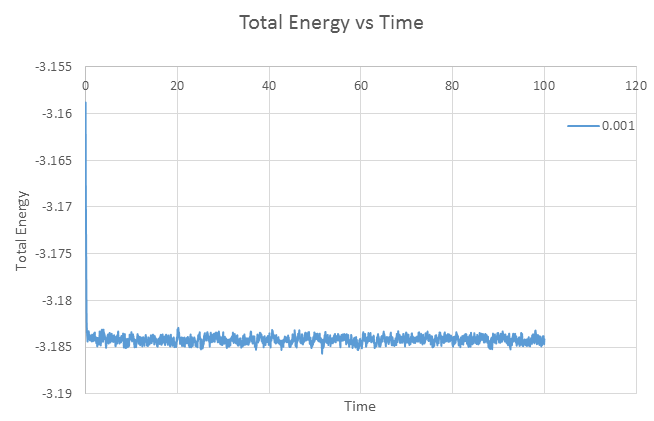
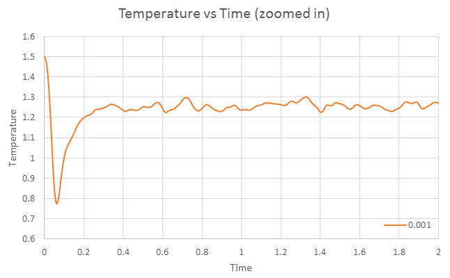
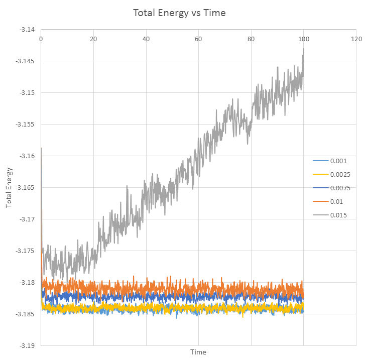
Make plots of the energy, temperature, and pressure, against time for the 0.001 timestep experiment (attach a picture to your report). Does the simulation reach equilibrium? How long does this take? When you have done this, make a single plot which shows the energy versus time for all of the timesteps (again, attach a picture to your report). Choosing a timestep is a balancing act: the shorter the timestep, the more accurately the results of your simulation will reflect the physical reality; short timesteps, however, mean that the same number of simulation steps cover a shorter amount of actual time, and this is very unhelpful if the process you want to study requires observation over a long time. Of the five timesteps that you used, which is the largest to give acceptable results? Which one of the five is a particularly bad choice? Why?
Equilibrium can be said to be achieved when thermodynamic quantities becomes constant. Hence for the timestep 0.001, the simulation reaches equilibrium since the plots of temperature and pressure versus time equilibrates to a constant value of approximately 1.25K and 1.25atm. From the zoomed in view, we can deduce that equilibration is achieved within 0.05s. Equilibrium has also been achieved for other timesteps, except 0.015, where the graph of total energy versus time graph is observed to gradually increase. The largest timestep to provide acceptable results is 0.01. Timestep 0.015 is a particularly bad choice because the simulation does not achieve equilibrium as its total energy value is increasing over time, with a large spread of error (larger fluctuation).
JC: If 0.01 is an acceptable choice, why do you decide to use 0.0025 in the next section? Should the average energy of the system depend on the choice of timestep (as it does for 0.0075 and 0.01)?
Graph of Total energy versus time for timestep 0.001
Graph of Temperature versus time for timestep 0.001
Graph of Temperature versus time for timestep 0.001, zoomed in version
Graph of Pressure versus time for timestep 0.001
Graph of Total Energy versus time for timesteps 0.001, 0.0025, 0.0075, 0.01, 0.015.
Part 4: Running simulations under specific conditions
Task 1
Choose 5 temperatures (above the critical temperature ![]() ), and two pressures (you can get a good idea of what a reasonable pressure is in Lennard-Jones units by looking at the average pressure of your simulations from the last section). This gives ten phase points — five temperatures at each pressure. Create 10 copies of npt.in, and modify each to run a simulation at one of your chosen
), and two pressures (you can get a good idea of what a reasonable pressure is in Lennard-Jones units by looking at the average pressure of your simulations from the last section). This gives ten phase points — five temperatures at each pressure. Create 10 copies of npt.in, and modify each to run a simulation at one of your chosen ![]() points. You should be able to use the results of the previous section to choose a timestep. Submit these ten jobs to the HPC portal. While you wait for them to finish, you should read the next section.
points. You should be able to use the results of the previous section to choose a timestep. Submit these ten jobs to the HPC portal. While you wait for them to finish, you should read the next section.
Temperatures used: 2.0, 2.5, 3.0, 3.5, 4.0
Pressures used: 2.5, 2.8
Timestep used: 0.0025
Task 2
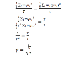
We need to choose ![]() so that the temperature is correct
so that the temperature is correct ![]() if we multiply every velocity
if we multiply every velocity ![]() . We can write two equations:
. We can write two equations:
![]()

Solve these to determine ![]() .
.
JC: Nearly, but the T and curly T in your answer are the wrong way round, T should be the denominator.
Task 3
Use the manual page to find out the importance of the three numbers 100 1000 100000. How often will values of the temperature, etc., be sampled for the average? How many measurements contribute to the average? Looking to the following line, how much time will you simulate?
A measurement will be made every '100' units, with '1000' defined to provide the total average of all the '100000' values.
JC: This is a bit unclear.
Task 4
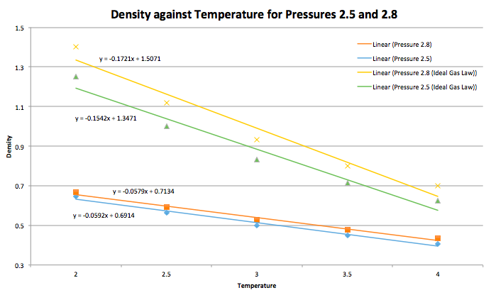
When your simulations have finished, download the log files as before. At the end of the log file, LAMMPS will output the values and errors for the pressure, temperature, and density ![]() . Use software of your choice to plot the density as a function of temperature for both of the pressures that you simulated. Your graph(s) should include error bars in both the x and y directions. You should also include a line corresponding to the density predicted by the ideal gas law at that pressure. Is your simulated density lower or higher? Justify this. Does the discrepancy increase or decrease with pressure?
. Use software of your choice to plot the density as a function of temperature for both of the pressures that you simulated. Your graph(s) should include error bars in both the x and y directions. You should also include a line corresponding to the density predicted by the ideal gas law at that pressure. Is your simulated density lower or higher? Justify this. Does the discrepancy increase or decrease with pressure?
Density in Ideal Gas Law calculation:
At any fixed pressure, the simulated density is lower than the ideal gas law plot. The ideal gas law states that there is negligible interaction between molecules, leading to no repulsive forces. Given this, molecules are more likely to be found next to one another, as compared to the simulation. Where in the case of a simulation, interactions between molecules are present, along with the presence of repulsion forces. This causes the molecules to be found far away from each other. Hence for a given volume, density is higher for an ideal gas (molecules near each other) than for a non-ideal gas (molecules far apart). This discrepancy of ideal gas law and simulation increases with pressure. This is because at high pressures, molecules are forced to be next to each other, increasing repulsion, therefore reducing density.
JC: How does the discrepancy between ideal gas and simulation results change with temperature?
Part 5: Calculating heat capacities using statistical physics
Task 1
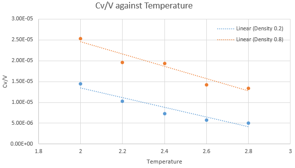
As in the last section, you need to run simulations at ten phase points. In this section, we will be in density-temperature ![]() phase space, rather than pressure-temperature phase space. The two densities required at 0.2 and 0.8, and the temperature range is 2.0, 2.2, 2.4, 2.6, 2.8. Plot
phase space, rather than pressure-temperature phase space. The two densities required at 0.2 and 0.8, and the temperature range is 2.0, 2.2, 2.4, 2.6, 2.8. Plot ![]() as a function of temperature, where
as a function of temperature, where ![]() is the volume of the simulation cell, for both of your densities (on the same graph). Is the trend the one you would expect? Attach an example of one of your input scripts to your report.
is the volume of the simulation cell, for both of your densities (on the same graph). Is the trend the one you would expect? Attach an example of one of your input scripts to your report.
The trend observed in the graph above is not what would normally be expected as Cv/V is supposed to increase with temperature. At higher temperatures, the total internal energy of the system increases, therefore higher heat capacity due to the increased difficulty to increase the temperature per unit. A lower density also leads to a lower heat capacity, lowering the height of the trendline. This is because heat capacity is an extensive property. A larger density would mean more atoms at the given fixed volume, hence driving up the Cv/V value.
JC: Why would you normally expect Cv/V to increase with temperature? Your explanation is not clear.
Input script for density 0.2 at temperature 2.0 attached: File:5.1 (0.2,2.0).in
Part 6: Structural properties and the radial distribution function
Task 1
Perform simulations of the Lennard-Jones system in the three phases. When each is complete, download the trajectory and calculate ![]() and
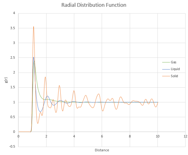
and ![]() . Plot the RDFs for the three systems on the same axes, and attach a copy to your report. Discuss qualitatively the differences between the three RDFs, and what this tells you about the structure of the system in each phase. In the solid case, illustrate which lattice sites the first three peaks correspond to. What is the lattice spacing? What is the coordination number for each of the first three peaks?
. Plot the RDFs for the three systems on the same axes, and attach a copy to your report. Discuss qualitatively the differences between the three RDFs, and what this tells you about the structure of the system in each phase. In the solid case, illustrate which lattice sites the first three peaks correspond to. What is the lattice spacing? What is the coordination number for each of the first three peaks?
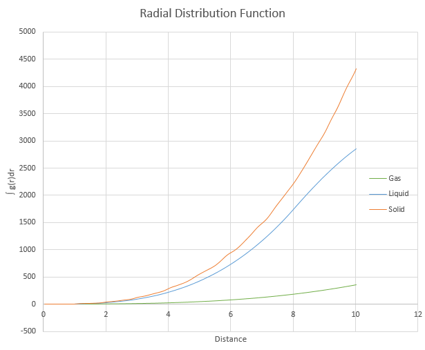
The number of peaks in the g(r) plot corresponds to the number of neighbouring atoms. As the solid has the highest number of peaks in the g(r) plot, it has the most neighbouring atoms, followed by liquid and finally gas. The distance between neighbouring atoms in a gas can be seen to be approximately a few times bigger than the solid as within a single gas peak, there are multiple solid peaks. The first 3 peaks for the solid corresponds to the 3 nearest atoms to the sampled atom, as per equidistant lattice points on a cube. The coordination number for the first three peaks are 12, 18 and 42.
JC: Did you calculate the lattice parameter for the solid? How did you obtain the coordination numbers? A plot of the RDF integral zoomed in at small r, and a diagram of an fcc unit cell with the 3 nearest neighbour atoms indicated would be good.
Part 7: Dynamical properties and the diffusion coefficient
Task 1
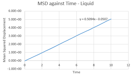
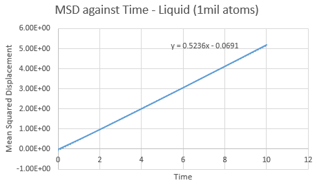
Make a plot for each of your simulations (solid, liquid, and gas), showing the mean squared displacement (the "total" MSD) as a function of timestep. Are these as you would expect? Estimate ![]() in each case. Be careful with the units! Repeat this procedure for the MSD data that you were given from the one million atom simulations.
in each case. Be careful with the units! Repeat this procedure for the MSD data that you were given from the one million atom simulations.
| 1 atom | 1 million atoms |
|---|---|
 |
|
 |
|
 |
|
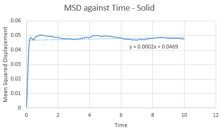
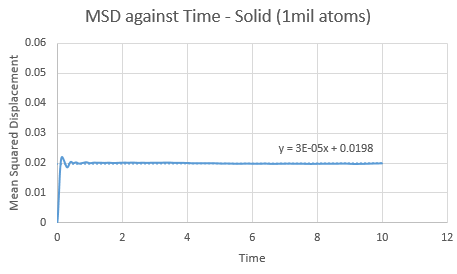
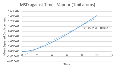
Trendline for 1 million liquid and vapour atoms has a larger gradient and intercept than the normal box simulation. This is opposed in the solid, with a lower gradient and intercept for the 1 million atoms. The observations in these trends are as expected.
The value of D can be found using the equation , where the
value can be found via gradient of each plot. By increasing the amount of total atoms, the diffusion coefficient increases for the liquid and gas, except for the solid. This is due to its high density property.
JC: To get the diffusion coefficient from the MSD a straight line should be fitted to only the linear part of the graph as this is when the simulation has reached the diffusive regime.
| LIQUID | 1 unit cell | 1 million atoms |
|---|---|---|
| Gradient | 0.5094 | 0.5236 |
| D | 0.0849 | 0.0873 |
| SOLID | 1 unit cell | 1 million atoms |
|---|---|---|
| Gradient | 2.00E-04 | 3.00E-05 |
| D | 3.33E-05 | 5.00E-06 |
| GAS | 1 unit cell | 1 million atoms |
|---|---|---|
| Gradient | 9.9061 | 15.249 |
| D | 1.65 | 2.54 |
Task 2
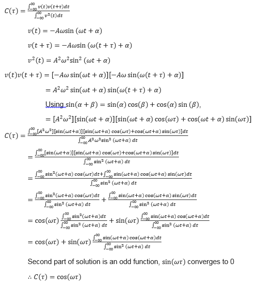
In the theoretical section at the beginning, the equation for the evolution of the position of a 1D harmonic oscillator as a function of time was given. Using this, evaluate the normalised velocity autocorrelation function for a 1D harmonic oscillator (it is analytic!):
 .
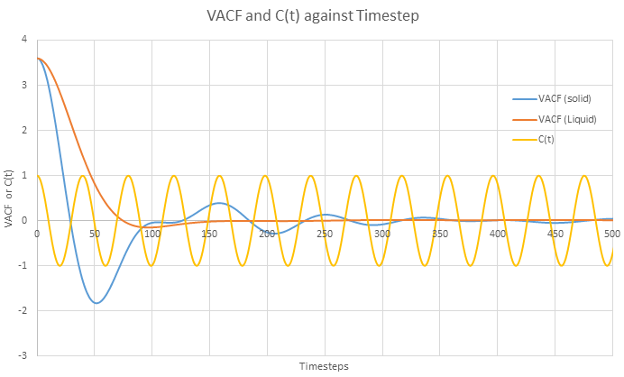
Be sure to show your working in your writeup. On the same graph, with x range 0 to 500, plot
 ![]() with
with ![]() and the VACFs from your liquid and solid simulations. What do the minima in the VACFs for the liquid and solid system represent? Discuss the origin of the differences between the liquid and solid VACFs. The harmonic oscillator VACF is very different to the Lennard Jones solid and liquid. Why is this? Attach a copy of your plot to your writeup.
and the VACFs from your liquid and solid simulations. What do the minima in the VACFs for the liquid and solid system represent? Discuss the origin of the differences between the liquid and solid VACFs. The harmonic oscillator VACF is very different to the Lennard Jones solid and liquid. Why is this? Attach a copy of your plot to your writeup.
JC: Good derivation.
