User:Msk315

Numerical answers to tasks mostly correct. Explanations could have been more thought out and better explained. The report would have benefited from a clear motivation and aim.

Report

Abstract

Molecular dynamics (MD) was used to simulate the detailed structural dynamics of simple liquid over a time based on an potential energy function. In this simulation, the Lennard-Jones potential function was used to approximate the strong force interactions "strong force" is not the right term to use here. We are definitely not modelling the strong nuclear force. If you are using strong as an adjective, it is not a correct description: LJ potentials model strong repulsive forces at short separations, but also attractive forces that tend to 0 at infinite separation (well, we use a cutoff). to simulate various physical properties of liquid, gas and solid. The heat capacity, radial distribution function, diffusion coefficient and total energy were calculated by considering every single particle in the simulation.

Introduction

Molecular dynamics (MD) was used to simulate the detailed structural dynamics of simple liquid over a time based on an grammar potential energy function.One of the key applications of molecular dynamic simulation is drug analysis, where the drug molecule binding to receptors and binding strength can be simulated microscopically by varying the binding strength of the protein structure It is a bit odd to single out drug analysis here, since your simulations of a LJ fluid/solid are not very relevant to this . In this lab we study through the use of large scale not large scale compared to the current standard - 1000 LJ atoms is very cheap numerical simulations of 1000 atoms to understand how various macroscopic properties of a system of particles change due to other particles. The simulation of the particles is done using the Velocity Verlet algorithm, an improved version of the Verlet algorithm tailored to simulate the velocities and position of every single particle the normal verlet could do this too . This is an example of using numerical methods to simulate physical systems that otherwise have analytical differential equations that are too computationally expensive to simulate analytically. Although we can in theory solve for a more accurate model of how particles behave by solving the Schrodinger equation for each particle and simulating them, we find that it’s much too complicated expensive . As such, we realize that utilizing the Lennard-Jones potential gives a very good approximation to the intermolecular forces and interactions.

The simulation uses roughly 1000 to 10,000 atoms as any more would be too computationally expensive and with 1000 atoms, we get a very good rough picture of how the particles behave. The initial velocity of each particle is chosen randomly from a Maxwell-Boltzmann Distribution, which describes how particles’ velocity varies according to a given temperature and mass. In order to calculate thermodynamic properties, we need to allow the system to reach equilibrium state, as most thermodynamic values are based off on grammar steady state systems.

Lastly, we utilize the NVT (Canonical) and NpT (Isobaric-isothermal) ensembles to describe how the particles will behave. These come from statistical mechanics and describes what macroscopic properties are kept constant. For example, total particle N, pressure, p and temperature are kept constant for the NpT ensemble.

In a scientific paper, the purpose of an introduction is to provide the reader with the necessary background theory, and to motivate the study. You have written a brief introduction to molecular dynamics, and included some information that would better placed in the methodology section (e.g. simulations were carried out in the NVT/NPT ensemble).

Aims and Objectives

Using these tools, It was aimed to determine the dynamic properties and diffusion coefficients of a simple liquid using molecular dynamic simulation. In order to do this, the density of the system, the variation of heat capacity with temperature, and the change in the radial distribution function were analysed.

In this lab, the fundamental understanding of how atoms interact due to intermolecular forces such as the Lennard-Jones potential was used to determine the dynamic and structural properties of various states of matter. Certain macroscopic properties of the simulated particles, such as the density, temperature were fixed and some extrinsic properties were simulated. The properties studied include how the density changes due to temperature at two pressure points. Calculating the heat capacity for 10 phase points in an NVT ensemble. Then the change of Radial Distribution Function (RDF) was studied depending on the displacement from a reference atom. Lastly the diffusion coefficient of a given system was analysed for the three phases using Mean Squared Displacement (MSD) methods and Velocity Autocorrelation Function (VACF) method. The simulation was performed using a specialized software LAMMPS, for molecular dynamics. Similar to your introduction, you tell the reader what you have done - this is what the methodology section is for.

Methods

In order to calculate diffusion and dynamic properties of a simple liquid, the simulations were performed using LAMMPS, where both Lennard-Jones potential well depth and zero-potential length were set to 1.0 in reduced units. The mass of a particle was set to 1.0 for simplicity. A cubic lattice of length 15 unit cells and number density 0.8 was melted in a certain temperature and pressure to form the desired state. The simulation was done in an NVE ensemble. The particle velocities were simulated randomly in a Monte-Carlo simulation and the velocity distribution based on a Boltzmann distribution.

Reduced units

In our simulation, we simplify the units used by using reduced units, these units simplify the numbers by scaling various variables according to atomic units used in the Lennard-Jones potential. They simplify the calculations by making most numbers simple integers of an order of 1, where both Lennard-Jones potential well depth and zero-potential length were set to 1.0 in reduced units. The mass of a particle was set to 1.0 for simplicity. A cubic lattice of length 15 unit cells and number density 0.8 was melted in a certain temperature and pressure to form the desired state. The simulation was done in an NVE ensemble. The particle velocities were simulated randomly in a Monte-Carlo simulation and the velocity distribution based on a Boltzmann distribution.

Determining a suitable timestep

An initial analysis of the timestep was done to roughly determine a suitable timestep to be used for the experiment. In computational experiments, larger timesteps trade off accuracy for speed, whilst low timesteps have high accuracy but is computationally expensive. By running a trial simulation in a variety of timesteps, it was found that the worst choice of timestep is 0.015 as it does not converge, whilst any timestep up to 0.0025 appears to be suitable.

Number Density vs Temperature

In this section we want to analyze how the density varies according to temperature and pressure. We choose two reduced pressure 2.5 and 2.7 in Lennard-Jones unit and plot them. The temperatures chosen are all above the critical temperature of 1.5.

As a comparison, we also overlay the graphs of the results together with that of the theoretical results derived from ideal gas law with the same reduced pressure units. This will give us deeper insight on the behavior and deviation of a Lennard-Jones gas from ideal gas behavior.

Measuring heat capacity

For the heat capacity, we utilize the NVT ensemble. This is because the desired thermodynamic property we're trying to simulate is the heat capacity at constant volume.

$C_V=\frac{\partial E}{\partial T}=\frac{\mathrm{V}\mathrm{a}\mathrm{r}\left[E\right]}{k_B{T}^2}=N^2\frac{⟨E^2⟩-{⟨E⟩}^2}{k_B{T}^2}$

We note from the above equation that the heat capacity can be computed statistically from a simulation, using the variance and average of the energy as well as its simulated temperature. Each energy has to be multiplied by N2 as LAMMPS outputs the energy per particle as opposed to the total energy.

This simulation is suitable to simulate the heat capacity of real particle systems because heat capacity is ultimately a macroscopic statistical property as opposed to a microscopic property, so statistical variance and averaging is generally a good idea.

Radial Distribution Function

The RDF is calculated using the VMD, the VMD enables us to analyze a given trajectory and output how the number density of a given particle system change with increasing displacement from a reference atom. The RDF was calculated for three phases, solid, liquid and gas and the integral was also performed. The RDF would serve to show some subtle physical properties of the lattice structures and the coordination numbers.

MSD Methodology

To calculate the diffusion coefficient, we need to use the relation of the MSD to the diffusion coefficient. $D=\frac{1}{6}\frac{\partial ⟨r^2\left(t\right)⟩}{\partial t}$

Two methods were used to extract a value for the diffusion coefficient for each phase. The first method leveraged on the line of best fit. The MSD was plot against the time and the line of best fit was drawn. From there, the gradient of the best fit line represented the derivative and we simply have to scale it to a sixth of its value to get the diffusion coefficient. There were some inefficiencies associated with this method. Namely that the simulation takes some amount of timesteps before the relationship becomes linear. As such the line of best fit has some errors associated with it. An alternate method utilized discrete differentiation. To calculate a derivative, the difference between two points in a timestep was calculated and divided by the timestep to get the gradient at each point. This numerical derivative was then plot against time. Similarly a line of best fit was drawn and the intercept was taken as a good approximation of the value of the diffusion coefficient.

VACF Methodology

For the VACF method, the data was plot against time, the curves for the three phases were also compared to that of the Harmonic Oscillator due to the Lennard-Jones potential. In order to calculate the Diffusion Coefficient, the trapezium rule was used to calculate the Diffusion Coefficient. As with all numerical methods, there are some errors associated with it. For curves that have a negative second derivative, the trapezium rule would give an underestimate, whilst a positive second derivative would result in an overestimate. Numerical integration was performed from the beginning to the end of the timestep. Using this formula, $D=\frac{1}{3}\underset{0}{\overset{\mathrm{\infty }}{\int }}\mathrm{d}\tau ⟨\mathbf{v}\left(0\right)\cdot \mathbf{v}\left(\tau \right)⟩$ A one-third scaling factor of the integration would give the diffusion coefficient.

The methodology section of a scientific paper aims to convey what you have done so that another scientist can reproduce your results, and to do this as concisely as possible. Information on e.g. what reduced units are is unnecessary. Equations for diffusion coefficients etc. are probably more at home in the introduction.

Results and Discussions

Number density as a function of temperature

molecule1
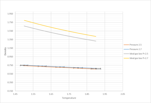Comparison between density under ideal gas behaviour and Lennard-Jones simulation

As shown in the graph, the density decreased as temperature increased. This was because of the expansion of the material. As temperature went up "went up" is not very scientific language , particles gained kinetic energy and grammar have collisions with the wall more frequently. However, because of the system setting, pressure stayed the same despite the rise in collision frequency. Surface area of the walls have increased as a result, and therefore, volume increased (i.e. density decreased as N was fixed). In comparison to results derived from the ideal gas law, it was shown that the simulated density was lower. This grammar was because ideal gas theory assumed that there were no interactions between molecules except during elastic collisions of negligible duration. Without taking repulsive interactions into account, molecules would be closer to each other (i.e. density would be higher) under ideal gas assumption. At a higher pressure (p=2.7), the discrepancy was even higher as molecules are forced to be closer to each other at higher pressure. They experience greater repulsive interactions. Therefore, their density was even lower.

Heat capacity as a function of temperature

molecule1
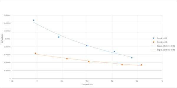$C_V/V$ as a function of temperature at density=0.2 and 0.8

The heat capacity of a system is the amount of heat needed to raise the system’s temperature by one degree. It was shown in the graph that the heat capacity decreased as temperature increased (i.e. less heat was required to heat up the system at higher temperature). This was because molecules have higher density of available energy states at higher temperature. As a result, the probability that a given state would be occupied was higher at an elevated temperature. One would expect that Cv is independent of T

Radial distribution function

molecule1	molecule1
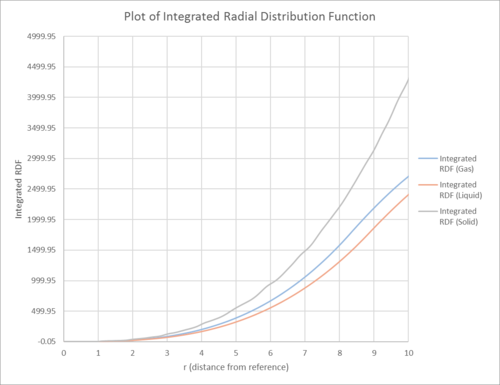The RDF against the distance from reference for solid, liquid and gas	The integral of the RDF against the distance from reference

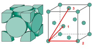
In this section, the structure of a system was simulated using radial distribution function g(r). The radial distribution function g(r) describes the density of particles from reference. For all the phases (solid, liquid and gas), the RDF is 0 at short distances, due to the interatomic repulsions at these distances. For solid, the RDF contained more maximum peaks relative to liquid and gas. Also, it asymptotically decayed into the value of 1 over a longer distance as opposed to the fluid phases. This observation was best evinced spelling by the periodicity of the atoms in the solid phase. (which enabled vibrational movement) This was reflected in the plot of the RDF graph which showed a series of concentric shells of increased and decreased densities surrounding the reference particles. The asymptotic value of 1 for the RDF was significant because it represented the bulk density of the substance. The slower approach of solid to the asymptotic value could also be explained by the different crystal structure. The solid had fcc structure (i.e. it had a higher number density) so was less homogenous over a small volume. It had 12, 6, 24 lattice points which were 1.114, 1.575, and 1.929 away from the reference lattice point.

molecule1	molecule1	molecule1
12 Lattice points equidistant from the blue reference lattice point	6 Lattice points equidistant from the blue reference lattice point	24 Lattice points equidistant from the blue reference lattice point

In contrast, for fluid phases much lesser maximas are observed and the RDF decays to one asymptotically much more rapidly. This can be explained by the relative strengths in intermolecular bond strength, allowing fluid molecules to move around more easily and lose their long range structures quickly. Despite the similarities in both gas and liquid phases as they are both fluid, the gas phase demonstrates an even less pronounced peak and oscillations due to the even weaker intermolecular forces.

Mean squared displacement

You should fit a straight line in the diffusive regime only. Also, you should be working in LJ units. Line of best fit gradient and intercept shown on graph stated to too many decimal places.

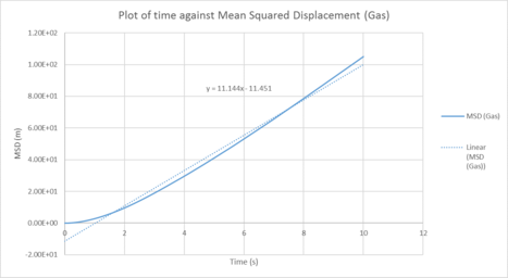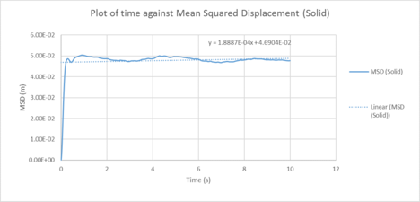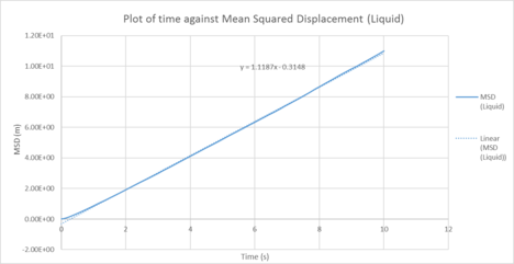
Plots of the Mean squared displacement against timestep for the solid, liquid and gas phases of our simulation

Table 1 : Calculated diffusion coefficients from the MSD for 1000 atom system

	D (line of best fit)	D (derivative)
gas	3.72 m2 / s	2.25 m2 / s
liquid	0.373 m2 / s	0.151 10-4 m2 / s
solid	1.0 x 10-4 m2 / s	3.19 x 10-3 m2 / s

Table 2 : Calculated diffusion coefficients from the MSD for 1,000,000 atom system

	D (line of best fit)	D (derivative)
gas	5.08 m2 / s	3.25 m2 / s
liquid	0.17 m2 / s	8.17 x 10-3 m2 / s
solid	6.40 x 10-6 m2 / s	1.33 x 10-3 m2 / s

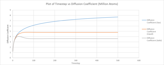
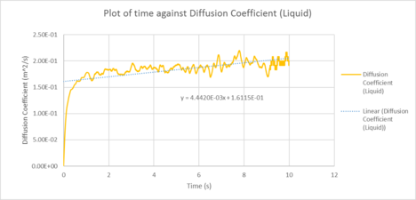
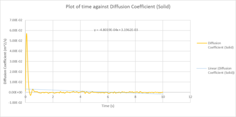
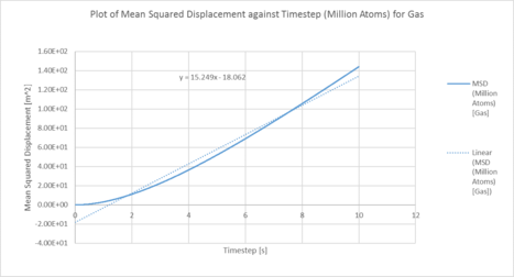
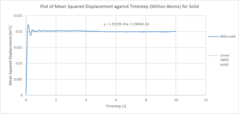
In statistical mechanics, the mean squared displacement (MSD) is a statistical measure of the spatial extent of random motion by particles. The diffusion coefficient indicates the rate of spread of the particles or the rate of coalescence if negative, and the diffusion coefficient is proportional to the derivative of the MSD. In general, the diffusion coefficient varies according to the phase of state in the order D(solid) < D(Liquid) < D(Gas). This was because gas systems had the lowest density (i.e. gas particles had the greatest diffusion mobility). Solid particles were in a fixed lattice and showed very little diffusion, so their diffusion coefficient converged to 0. It can be observed that in general, for the two methodologies applied to calculate the diffusion coefficient. The method that used the numerical derivative had a much better agreement with the values obtained from the VACF. This was to be expected as the derivative approach had less errors associated with that of the best fit line. For the data on the gas, since the MSD plot never reached a sufficiently linear relationship in the given timesteps, the end point of the derivative was used instead as a line of best fit was not a suitable form of analysis. This is not well communicated: what do you mean by the "end point of the derivative"? Do you mean the derivative value at the last time step? This is not a good idea, the derivative is very noisy.The values correspond quite well with each other. This was true for both the simulated data and the million atoms data.

Velocity auto-correlation function

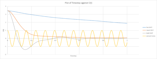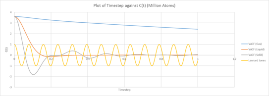
Plot of VACF for the gas, liquid and solid phases against time (left: our simulation, right: provided data for 1,000,00 atoms)

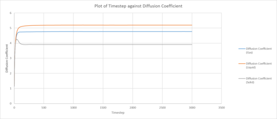
Plot of running VACF integrals for each phase against time (left: our simulation, right: provided data for 1,000,00 atoms)

The Velocity Autocorrelation Function measures how the velocity of a later time correlates with that of the current velocity. As the timestep approaches infinity, we expect the correlation to approach zero asymptotically. This is because we expect that the velocity at a much later time to be much less correlated with that of the current velocity. This is evident in the plot of the VACF against the timestep.

We observe that the correlation decreases much faster for liquids and solids than that for gas. This can be understood in terms of intermolecular forces. Molecules in the vapor state experiences little molecular forces as such any changes in motion and velocity is due to mostly random fluctuations. There isn’t an active agent changing how the velocity varies over time. Whilst for liquids and solids, the intermolecular forces are evidently much stronger and these interactions between the different molecules causes the change in velocity to vary much faster, and hence exhibit much lower correlation over a shorter timescale. This difference in interaction and intermolecular forces can be understood in by analyzing the electromagnetic Coulomb force and the strong force, approximated with the Lennard-Jones potential. The the strong force only acts in very close distances and has a short range, as such it is completely negligible for gases, and slightly less so for liquids. Coulombic forces exhibit an inverse square law and the greater the mean separation, the weaker the interaction. This is accounted for in the simulation by the density. A decreased density indicates a generally longer intermolecular separation and a higher Mean Separation Displacement as shown in the previous sections. As a result, the Coulomb Force is much weaker acting on liquids and even less so for vapor states. There are no permanent charges in the system. The LJ potential models the interaction between two neutral species. Solid atoms are more fixed on positions (i.e. they are located in the well of Lennard-Jones potential). Therefore, they do not move far from their positions but oscillate back and forth. Another way to think about this is to consider the potential energy of the nucleus due to the attractive region of the Lennard-Jones potential combined with the repulsive part of the Coulomb potential. The LJ repulsive wall models Pauli repulsion attractive part is dispersion. For solids, the separation of that scale, the molecules usually lie within the minima of the potential. As we understand it, motion about that region can be approximated to exhibit simple harmonic motion about the minima, resulting in vibrational motion. For the liquid phase, the motion of the particles still has some semblance to that of oscillatory motion, we can understand that in terms of anharmonicity. For much large molecular separations between atoms, the Taylor expansion along the minima can no longer be approximated as a simple quadratic potential, as such anharmonic motion occurs. Whilst gas phases, where the separation is far from the attractive region, they would not exhibit the same type of vibrational motion seen in solids. With gas molecules being essentially free particles that is essentially unencumbered by the intermolecular forces. The minima of the VACF functions for solids and liquids describe when the particles have the maximum velocity in the opposite direction. This corresponds to when they are passing through the center and have zero acceleration. remember VACF incorporates statistics from all the particles. Do they all reverse velocity at the same time? The VACF graph of solids and liquids differ from that of the Harmonic VACF function for a few reasons. The most poignant reason being that simple harmonic motion is a much more simplified model for only 2 particles, the energy is contained within 2 atoms in a closed system and the potential is exactly quadratic. Whilst for the simulations, we note that the Lennard-Jones potential is not exactly a quadratic function, additionally there can be momentum and energy transfer between different molecules due to collisions and energy is lost.

Conclusions

Looking at the results, we can observe that most of the simulation corresponds well with known physical laws based on the in built mechanisms that we used for the simulations. All deviations from the expected trends can be explained through known scientific laws, such as the deviation from ideal gas behavior for the number density section, the correlation between heat capacity and temperature, and lastly the difference in diffusion coefficients with respect to the phase that the system is in.

Naturally the next step to be done would be to compare these simulations with real experimental data to validate the veracity and usefulness of the simulations. Another future point of work would be to use a more physically accurate and meaningful model. For example instead of using the Lennard-Jones Potential, the Saxon-Woods potential could be considered to model it more accurately. Other physical phenomena could also be modelled into the simulation model, such as the inclusion of Coulombic forces.

There are other macroscopic variables that may also be of interest and is well within the means of the current simulation model to predict, for example the viscosity of the particles or convection could be simulated in future works.

Tasks

TASK: Open the file HO.xls.

In it, the velocity-Verlet algorithm is used to model the behaviour of a classical harmonic oscillator. Complete the three columns "ANALYTICAL", "ERROR", and "ENERGY": "ANALYTICAL" should contain the value of the classical solution for the position at time $t$, "ERROR" should contain the absolute difference between "ANALYTICAL" and the velocity-Verlet solution (i.e. ERROR should always be positive -- make sure you leave the half step rows blank!), and "ENERGY" should contain the total energy of the oscillator for the velocity-Verlet solution. Remember that the position of a classical harmonic oscillator is given by $x\left(t\right)=A\cos (\omega t+\varphi )$ (the values of $A$, $\omega$, and $\varphi$ are worked out for you in the sheet).

TASK: For the default timestep value, 0.1, estimate the positions of the maxima in the ERROR column as a function of time. Make a plot showing these values as a function of time, and fit an appropriate function to the data.

TASK: Experiment with different values of the timestep. What sort of a timestep do you need to use to ensure that the total energy does not change by more than 1% over the course of your "simulation"? Why do you think it is important to monitor the total energy of a physical system when modelling its behaviour numerically?

Time step: 0.02
When simulating a physical system's diffusion and dynamic properties, it is crucial to monitor the total energy of the system, as it tells you whether the system is in thermal equilbrium or not (i.e. whether energy is being conserved or not). Therefore, it is important to select a timestep that gives a compromise between simulation complexity and minimal error.

TASK: For a single Lennard-Jones interaction,

$\varphi \left(r\right)=4ϵ(\frac{{\sigma }^{12}}{r^{12}}-\frac{{\sigma }^6}{r^6})$, find the separation, $r_0$, at which the potential energy is zero.

$r_0=\sigma$

What is the force at this separation?

$\frac{24ϵ}{r{0}_{}}$

Find the equilibrium separation, $r_{eq}$, and work out the well depth ($\varphi \left(r_{eq}\right)$).

$r_{eq}=\sqrt[6]{2r^6}$ and $\varphi \left(r_{eq}\right)=-ϵ$

Evaluate the integrals $\underset{2\sigma }{\overset{\mathrm{\infty }}{\int }}\varphi \left(r\right)\mathrm{d}r$, $\underset{2.5\sigma }{\overset{\mathrm{\infty }}{\int }}\varphi \left(r\right)\mathrm{d}r$, and $\underset{3\sigma }{\overset{\mathrm{\infty }}{\int }}\varphi \left(r\right)\mathrm{d}r$ when $\sigma =ϵ=1.0$.

$\underset{2\sigma }{\overset{\mathrm{\infty }}{\int }}\varphi \left(r\right)\mathrm{d}r=-0.0248$

$\underset{2.5\sigma }{\overset{\mathrm{\infty }}{\int }}\varphi \left(r\right)\mathrm{d}r=-8.178\times 10^{-3}$

$\underset{3\sigma }{\overset{\mathrm{\infty }}{\int }}\varphi \left(r\right)\mathrm{d}r=-3.29\times 10^{-3}$

It is shown that the integral (i.e. the force interaction between two particles) tends to 0 as the difference between the upper and the lower boundary condition increases. As the interparticle distance decreases, the interaction rises.

TASK: Estimate the number of water molecules in 1ml of water under standard conditions.

Estimate the volume of  10,000 water molecules under standard conditions.

Density of water = $1\frac{g}{c{m}^3}$
Molar mass of water = $18\frac{g}{mo{l}^{-1}}$

Mass of water in 1 mL = $1\frac{g}{c{m}^3}\times 1mL=1g$

Number of moles in 1 mL = $\frac{1}{18}mol$

Number of water molecules in 1 mL =$6.023\times 10^{23}\times \frac{1}{18}=3.35\times 10^{22}(3.s.f)$

$3.35\times 10^{22}$ water molecules : 1 mL = $10000$ water molecules: $x$

$x=\frac{10000}{3.35\times 10^{22}}=2.99\times 10^{-19}mL(3.s.f)$

Regarding experimental efficiency, 1mL is a realistic volume. However, the number of water molecules ( $3.35\times 10^{22}$ ) is too huge for efficient simulation. Then again, when simulating only 10,000 water molecules, $2.99\times 10^{-19}mL$ is not a realistic volume.

TASK: Consider an atom at position

$(0.5,0.5,0.5)$ in a cubic simulation box which runs from $(0,0,0)$ to $(1,1,1)$. In a single timestep, it moves along the vector $(0.7,0.6,0.2)$. At what point does it end up, after the periodic boundary conditions have been applied?.

Position before periodic boundary conditions applied = $(0.5,0.5,0.5)+(0.7,0.6,0.2)=(1.2,1.1,0.7)$

Position after periodic boundary conditions applied = $(0.2,0.1,0.7)$

The atoms are enclosed in a box of fixed dimensions. The periodic boundary condition is applied to ensure that when an atom passes out the boundary another atom passes through into the boundary so that the number of atoms in the box stays constant.

TASK: The Lennard-Jones parameters for argon

are $$\begin{gathered} \sigma =0.34\mathrm{n}\mathrm{m},ϵ \\ / \\ {k}_B=120\mathrm{K} \end{gathered}$$. If the LJ cutoff is $r^{*}=3.2$, what is it in real units? What is the well depth in $$\begin{gathered} {\mathrm{k}\mathrm{J} \\ \mathrm{m}\mathrm{o}\mathrm{l}}^{-1} \end{gathered}$$? What is the reduced temperature $T^{*}=1.5$ in real units?

distance $r^{*}=\frac{r}{\sigma }$

$r=3.2\times 0.34\times 10^{-9}=1.09\times 10^{-9}m=1.09nm$ energy $E^{*}=\frac{E}{ϵ}$

$U\left({{\mathbf{r}}_{\mathbf{(}}\mathbf{e}\mathbf{q}\mathbf{)}}^N\right)=-ϵ$

Therefore

$ϵ=-120K\times 1.38\times 10^{-23}=1.66\times 10^{-21}J(3.s.f)=0.997KJ/mol$

temperature $T^{*}=\frac{k_{B}T}{ϵ}$

$T=\frac{1.5\times 1.66\times 10^{-21}}{1.38\times 10^{-23}}=180K$

TASK: Why do you think giving atoms random starting coordinates causes problems in simulations?

Hint: what happens if two atoms happen to be generated close together?

This may cause problems because if two atoms happen to be generated close together the coordinates could overlap. This will cause problems with defining some properties of the atoms. Yes, when two atoms are generated close to each other they "overlap" (well, LJ models point masses), which corresponds to a very small separation, and extremely high interaction energy ==> extremely large repulsive force. The system would "explode" unless you use an extremely small time step, which is of course needlessly expensive. I'm not sure what you mean by your last sentence.

TASK: Satisfy yourself that this lattice spacing corresponds to a number density of lattice points of . Consider instead a face-centred cubic lattice with a lattice point number density of 1.2. What is the side length of the cubic unit cell?

$\text{Volume}=1.07722^3=1.25uni{t}^3$

$\text{Number density}=\frac{\text{Number of lattice points per unit cell}}{\text{Unit volume}}=\frac{1}{1.25}=0.8(1.d.p)$

$1.2=\frac{\text{Number of lattice points per unit cell}}{\text{Unit volume}}=\frac{4}{V}$

$\text{Volume of cubic unit cell}=\frac{4}{1.2}$

$\text{Side Length of the cubic unit cell}=\sqrt[3]{\frac{4}{1.2}}=1.49(3.s.f)$

TASK: Consider again the face-centred cubic lattice from the previous task.

How many atoms would be created by the create_atoms command if you had defined that lattice instead?

A simple cubic lattice has one lattice point per unit cell whereas a face-centred cubic lattice has 4 lattice points per unit cell. Therefore if in the simple cubic lattice 1 box creates 1000 atoms in a face-centered lattice 1 box will create 4000 atoms.

TASK: Using the LAMMPS manual, find the purpose of the following commands in the input script:

mass 1 1.0
pair_style lj/cut 3.0
pair_coeff * * 1.0 1.0

mass 1 1.0: This line is defining an atom of type 1 with a mass 1.0.

pair_style lj/cut 3.0: This is a set of formula(s) used to compute pairwise interactions. In LAMMPS, the pair potential is defined within a cutoff distance and the set of active interactions change over time. Therefore this code defines the cutoff as a distance of 3.0.

pair_coeff * * 1.0 1.0: Specifies the pair wise force field interaction for one or more atom types. The two asterisks correspond to two atoms of any type in the system. The two numbers at the end correspond to two coefficients in this case $\sigma =ϵ=1.0$.

TASK: Given that we are specifying ${\mathbf{x}}_i\left(0\right)$ and ${\mathbf{v}}_i\left(0\right)$, which integration algorithm are we going to use?

The velocity-Verlet algorithm

TASK: Look at the lines below.

### SPECIFY TIMESTEP ###
variable timestep equal 0.001
variable n_steps equal floor(100/${timestep})
timestep ${timestep}

### RUN SIMULATION ###
run ${n_steps}
run 100000

The second line (starting "variable timestep...") tells LAMMPS that if it encounters the text ${timestep} on a subsequent line, it should replace it by the value given. In this case, the value ${timestep} is always replaced by 0.001. In light of this, what do you think the purpose of these lines is? Why not just write:

timestep 0.001
run 100000

Ask the demonstrator if you need help.

TASK: make plots of the energy, temperature, and pressure, against time for the 0.001 timestep experiment (attach a picture to your report).

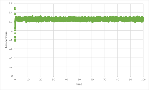
Does the simulation reach equilibrium? How long does this take? When you have done this, make a single plot which shows the energy versus time for all of the timesteps (again, attach a picture to your report). Choosing a timestep is a balancing act: the shorter the timestep, the more accurately the results of your simulation will reflect the physical reality; short timesteps, however, mean that the same number of simulation steps cover a shorter amount of actual time, and this is very unhelpful if the process you want to study requires observation over a long time. Of the five timesteps that you used, which is the largest to give acceptable results? Which one of the five is a particularly bad choice? Why?

molecule1	molecule1
plot of total energy against time for timestep 0.001	plot of temperature against time for timestep 0.001
molecule1
plot of the pressure against time for timestep 0.001

Total energy against time for varying timesteps

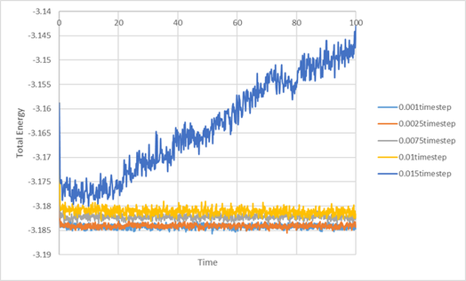
The time step 0.001 reached equilibrium within 0.2 seconds. 0.0025 time step also reached equilibrium in a similar time frame. It was the largest time step which gave acceptable results. With the time step 0.01 and 0.0075, the total energy did tend towards equilibrium, but not within a sensible time frame. The worst choice of time step would be the 0.015, as the total energy increased instead of tending towards equilibrium. The 0.015 time step should not be used as it causes the simulation to become unstable, and causes it not to converge to equilibrium.

TASK: Choose 5 temperatures (above the critical temperature $T^{*}=1.5$), and two pressures

(you can get a good idea of what a reasonable pressure is in Lennard-Jones units by looking at the average pressure of your simulations from the last section). This gives ten phase points — five temperatures at each pressure. Create 10 copies of npt.in, and modify each to run a simulation at one of your chosen $(p,T)$ points. You should be able to use the results of the previous section to choose a timestep. Submit these ten jobs to the HPC portal. While you wait for them to finish, you should read the next section.

$T^{*}=1.5,1.6,1.7,1.8,1.9$

$P=2.5,2.7$
$timestep:0.001$

TASK: We need to choose $\gamma$ so that the temperature is correct $T=\mathfrak{𝔗}$ if we multiply every velocity $\gamma$. We can write two equations:

$\frac{1}{2}\sum _i{m}_i{v}_i^2=\frac{3}{2}N{k}_{B}T$

$\frac{1}{2}\sum _i{m}_i{\left(\gamma v_i\right)}^2=\frac{3}{2}N{k}_B\mathfrak{𝔗}$

Solve these to determine $\gamma$

The equation that gives desired energy at modified velocitiy:

$\frac{1}{2}\sum _i{m}_i(v_i\gamma {)}^2=\frac{3}{2}N{k}_B\mathfrak{𝔗}$

${\gamma }^2\frac{1}{2}\sum _i{m}_i(v_i{)}^2=\frac{3}{2}N{k}_B\mathfrak{𝔗}$

${\gamma }^2\frac{3}{2}N{k}_{B}T=\frac{3}{2}N{k}_B\mathfrak{𝔗}$

Rearrangement gives: $\gamma =\pm \sqrt{\frac{\mathfrak{𝔗}}{T}}$

TASK: Use the manual page to find out the importance of the three numbers 100 1000 100000.

How often will values of the temperature, etc., be sampled for the average? How many measurements contribute to the average? Looking to the following line, how much time will you simulate?

100: Nevery, meaning the spacing between the time step values that will be used to calculate average. In our case, it is set to 100 so LAMMPS would take data sample every 0.001 timestep.
1000: Nrepeat, meaning the number of input values that will be used to calculate the average.
100000: Nfreq. This instructs LAMMPS to calculate the final average of all the previous averages after 100000 time steps.
To sum up, the average of temperature will be sampled every 100000 timestep with a 100 time step interval. 1000 measurements would contribute to the average.

TASK: When your simulations have finished, download the log files as before.

At the end of the log file, LAMMPS will output the values and errors for the pressure, temperature, and density $\left(\frac{N}{V}\right)$. Use software of your choice to plot the density as a function of temperature for both of the pressures that you simulated. Your graph(s) should include error bars in both the x and y directions. You should also include a line corresponding to the density predicted by the ideal gas law at that pressure. Is your simulated density lower or higher? Justify this. Does the discrepancy increase or decrease with pressure?

molecule1	molecule1
Density against reduced temperature with error bars	Comparison between density under ideal gas behaviour and Lennard-Jones simulation

As shown in the graph, the density decreased as temperature increased. This was because of the expansion of the material. As temperature went up, particles gained kinetic energy and have collisions with the wall more frequently. However, because of the system setting, pressure stayed the same despite the rise in collision frequency. Surface area of the walls have increased as a result, and therefore, volume increased (i.e. density decreased as N was fixed). In comparison to results derived from the ideal gas law, it was shown that the simulated density was lower. This was because ideal gas theory assumed that there were no interactions between molecules except during elastic collisions of negligible duration. Without taking repulsive interactions into account, molecules would be closer to each other (i.e. density would be higher) under ideal gas assumption. At a higher pressure (p=2.7), the discrepancy was even higher as molecules are forced to be closer to each other at higher pressure. They experience greater repulsive interactions. Therefore, their density was even lower. If you simulated higher temperatures of LJ, it would approach the ideal gas.

TASK: As in the last section, you need to run simulations at ten phase points.

In this section, we will be in density-temperature $({\rho }^{*},T^{*})$ phase space, rather than pressure-temperature phase space. The two densities required at $0.2$ and $0.8$, and the temperature range is $2.0,2.2,2.4,2.6,2.8$. Plot $C_V/V$ as a function of temperature, where $V$ is the volume of the simulation cell, for both of your densities (on the same graph). Is the trend the one you would expect? Attach an example of one of your input scripts to your report.

molecule1
$C_V/V$ as a function of temperature at density=0.2 and 0.8

The heat capacity of a system is the amount of heat needed to raise the system’s temperature by one degree. It was shown in the graph that the heat capacity decreased as temperature increased (i.e. less heat was required to heat up the system at higher temperature). This was because molecules have higher density of available energy states at higher temperature. As a result, the probability that a given state would be occupied was higher at temperature. The heat capacity is defined as:
$C_{\text{V}}={\left(\frac{\partial U}{\partial T}\right)}_{\text{V}}=\frac{3}{2}nR$

$PV=nRT$

$\frac{PV}{T}=nR$

$C_{\text{V}}=\frac{3PV}{2T}$

Therefore,

$\frac{C_{\text{V}}}{V}=\frac{3P}{2T}$

Cv/Vol is inversely proportional to 1/T. It was also shown in the graph that the heat capacity increased with density. At higher density, more molecules were found per volume, so there were more energy states to excite (i.e. more heat was required to heat up the system to a higher temperature).

An example of the input script (density=0.2, T=2.0)

### DEFINE SIMULATION BOX GEOMETRY ###
variable density equal 0.2

lattice sc ${density}
region box block 0 15 0 15 0 15
create_box 1 box
create_atoms 1 box

### DEFINE PHYSICAL PROPERTIES OF ATOMS ###
mass 1 1.0
pair_style lj/cut/opt 3.0
pair_coeff 1 1 1.0 1.0
neighbor 2.0 bin

### SPECIFY THE REQUIRED THERMODYNAMIC STATE ###
variable T equal 2.0
variable timestep equal 0.0010

### ASSIGN ATOMIC VELOCITIES ###
velocity all create ${T} 12345 dist gaussian rot yes mom yes

### SPECIFY ENSEMBLE ###
timestep ${timestep}
fix nve all nve

### THERMODYNAMIC OUTPUT CONTROL ###
thermo_style custom time etotal temp press
thermo 10

### RECORD TRAJECTORY ###
dump traj all custom 1000 output-1 id x y z

### SPECIFY TIMESTEP ###

### RUN SIMULATION TO MELT CRYSTAL ###
run 10000
unfix nve
reset_timestep 0

### BRING SYSTEM TO REQUIRED STATE ###
variable tdamp equal ${timestep}*100
fix nvt all nvt temp ${T} ${T} ${tdamp}
run 10000
unfix nvt
fix nve all nve
reset_timestep 0

### MEASURE SYSTEM STATE ###
thermo_style custom step etotal temp atoms 
variable x2 equal atoms*atoms
variable energy equal etotal
variable energy2 equal etotal*etotal
variable temp equal temp
variable temp2 equal temp*temp
variable x equal atoms

fix aves all ave/time 100 1000 100000 v_energy v_energy2 v_temp v_temp2 
run 100000

variable CV equal (((f_aves[2]-f_aves[1]*f_aves[1])/(f_aves[4]))*${x2})
variable avt equal f_aves[3]

print "Temperature: ${avt}"
print "Heat Capacity: ${CV}"
print "Atoms: ${Number}

TASK: When each is complete, download the trajectory and calculate $g(r)$ and $\int g(r)\mathrm{d}r$.

Plot the RDFs for the three systems on the same axes, and attach a copy to your report. Discuss qualitatively the differences between the three RDFs, and what this tells you about the structure of the system in each phase. In the solid case, illustrate which lattice sites the first three peaks correspond to. What is the lattice spacing? What is the coordination number for each of the first three peaks?

molecule1	molecule1
The RDF against the distance from reference for solid, liquid and gas	The integral of the RDF against the distance from reference

In this section, the structure of a system was simulated using radial distribution function g(r). The radial distribution function g(r) describes the density of particles from reference. For all the phases (solid, liquid and gas), the RDF is 0 at short distances, due to the interatomic repulsions at these distances.
For solid, the RDF contained more maximum peaks relative to liquid and gas. Also, it asymptotically decays into the value of 1 over a longer distance as opposed to the fluid phases. This observation is best evinced by the periodicity of the atoms in the solid phase. (which enables vibrational movement) This is reflected in the plot of the RDF graph which shows a series of concentric shells of increased and decreased densities surrounding the reference particles. The asymptotic value of 1 for the RDF is significant because it represents the bulk density of the substance. The slower approach of solid to the asymptotic value can also be explained by the different crystal structure.
In contrast, for fluid phases much lesser maximas are observed and the RDF decays to one asymptotically much more rapidly. This can be explained by the relative strengths in intermolecular bond strength, allowing fluid molecules to move around more easily and lose their long range structures quickly. Despite the similarities in both gas and liquid phases as they are both fluid, the gas phase demonstrates an even less pronounced peak and oscillations due to the even weaker intermolecular forces.

The lattice spacing is 1.575 based on the density 1.024 and N=4 (fcc). The first 3 peaks of the solid RDF correspond to 3 lattice points, which are 1.114, 1.575 and 1.929 (3 s.f.) away.

molecule1
3 Lattice points from the reference

	lattice point 1	lattice point 2	lattice point 3
Distance	1.114	1.575	1.929
Coordination number	12	6	24

molecule1	molecule1	molecule1
12 Lattice points equidistant from the blue reference lattice point	6 Lattice points equidistant from the blue reference lattice point	24 Lattice points equidistant from the blue reference lattice point

TASK: make a plot for each of your simulations (solid, liquid, and gas), showing the mean squared displacement (the "total" MSD) as a function of timestep.

Are these as you would expect? Estimate D in each case. Be careful with the units! Repeat this procedure for the MSD data that you were given from the one million atom simulations.

Plots of the Mean squared displacement against timestep for the solid, liquid and gas phases of our simulation

Plots of the Diffusion Coefficient against timestep for the solid, liquid and gas phases of our simulation

	D (line of best fit)	D (derivative)
gas	3.72 m2 / s	2.25 m2 / s
liquid	0.373 m2 / s	0.151 10-4 m2 / s
solid	1.0 x 10-4 m2 / s	3.19 x 10-3 m2 / s

One million system:

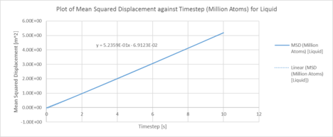
Plots of the Mean squared displacement against timestep for the solid, liquid and gas phases of simulation of a million atoms

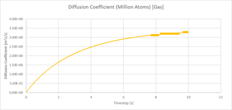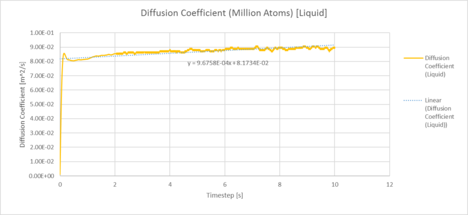
Plots of the Diffusion Coefficient against timestep for the solid, liquid and gas phases of simulation of a million atoms

	D (line of best fit)	D (derivative)
gas	5.08 m2 / s	3.25 m2 / s
liquid	0.17 m2 / s	8.17 x 10-3 m2 / s
solid	6.40 x 10-6 m2 / s	1.33 x 10-3 m2 / s

In statistical mechanics, the mean squared displacement (MSD) is a statistical measure of the spatial extent of random motion by particles. The diffusion coefficient indicates the rate of spread of the particles or the rate of coalescence if negative, and the diffusion coefficient is proportional to the derivative of the MSD. In general, the diffusion coefficient varies according to the phase of state in the order D(solid) < D(Liquid) < D(Gas). This was because gas systems had the lowest density (i.e. gas particles had the greatest diffusion mobility). Solid particles were in a fixed lattice and showed very little diffusion, so their diffusion coefficient converged to 0. It can be observed that in general, for the two methodologies applied to calculate the diffusion coefficient. The method that used the numerical derivative had a much better agreement with the values obtained from the VACF. This was to be expected as the derivative approach had less errors associated with that of the best fit line. For the data on the gas, since the MSD plot never reached a sufficiently linear relationship in the given timesteps, the end point of the derivative was used instead as a line of best fit was not a suitable form of analysis. The values correspond quite well with each other. This was true for both the simulated data and the million atoms data.

Fit straight line to diffusive regime only.

TASK: In the theoretical section at the beginning, the equation for the evolution of the position of a 1D harmonic oscillator as a function of time was given.

Using this, evaluate the normalised velocity autocorrelation function for a 1D harmonic oscillator (it is analytic!): $C\left(\tau \right)=\frac{\underset{-\mathrm{\infty }}{\overset{\mathrm{\infty }}{\int }}v\left(t\right)v(t+\tau )\mathrm{d}t}{\underset{-\mathrm{\infty }}{\overset{\mathrm{\infty }}{\int }}{v}^2\left(t\right)\mathrm{d}t}$

Be sure to show your working in your writeup. On the same graph, with x range 0 to 500, plot $C\left(\tau \right)$ with $\omega =1/2\pi$ and the VACFs from your liquid and solid simulations. What do the minima in the VACFs for the liquid and solid system represent? Discuss the origin of the differences between the liquid and solid VACFs. The harmonic oscillator VACF is very different to the Lennard Jones solid and liquid. Why is this? Attach a copy of your plot to your writeup.

Differentiation of our equation for the 1D harmonic oscillator ($x\left(t\right)=A\cos (\omega t+\varphi )$) with respect to time gives:

$\frac{\partial x}{\partial t}=v\left(t\right)=-\omega A\sin (\omega t+\varphi )$

Plugging back into the normalised VACF function

$C\left(\tau \right)=\frac{\underset{-\mathrm{\infty }}{\overset{\mathrm{\infty }}{\int }}{\omega }^2{A}^2\sin (\omega t+\varphi )\sin (\omega (t+\tau )+\varphi )\mathrm{d}t}{\underset{-\mathrm{\infty }}{\overset{\mathrm{\infty }}{\int }}(-\omega A\sin (\omega t+\varphi ){)}^2\mathrm{d}t}$

Simplifying the algebra:

$C\left(\tau \right)=\frac{\underset{-\mathrm{\infty }}{\overset{\mathrm{\infty }}{\int }}\sin (\omega t+\varphi )\sin (\omega (t+\tau )+\varphi )\mathrm{d}t}{\underset{-\mathrm{\infty }}{\overset{\mathrm{\infty }}{\int }}{\sin }^2(\omega t+\varphi )\mathrm{d}t}$

Using the product sum identity $\sin u\sin v=\frac{1}{2}[\cos (u-v)-\cos (u+v))]$

Similarly using the double angle formula, $si{n}^{2}u=\frac{1-\cos (2u))}{2}$ .

Substituting these in and simplifying:

$C\left(\tau \right)=\frac{\underset{-\mathrm{\infty }}{\overset{\mathrm{\infty }}{\int }}\cos (-\omega \tau )-\cos (2\omega t+\omega \tau +2\varphi )\mathrm{d}t}{\underset{-\mathrm{\infty }}{\overset{\mathrm{\infty }}{\int }}1-\cos (2\omega t+2\varphi )\mathrm{d}t}$

Integration with respect to t gives:

$C\left(\tau \right)={\left[\frac{t\cos (-\omega \tau )-\frac{1}{2\omega }\sin (2\omega t+\omega \tau +2\varphi )}{t-\frac{1}{2\omega }\sin (2\omega t+2\varphi )}\right]}_{-\mathrm{\infty }}^{\mathrm{\infty }}$

In order to evaluate our expression successfully, we then divide the top and bottom by t:

$C\left(\tau \right)={\left[\frac{\cos (-\omega \tau )-\frac{1}{2\omega t}\sin (2\omega t+\omega \tau +2\varphi )}{1-\frac{1}{2\omega t}\sin (2\omega t+2\varphi )}\right]}_{-\mathrm{\infty }}^{\mathrm{\infty }}$

and calculate our interval. This gives us:

$C\left(\tau \right)=\frac{\cos (-\omega \tau )-0}{1-0}$

which can be simplified to $C\left(\tau \right)=\cos (\omega \tau )$

Plot of VACF for the gas, liquid and solid phases against time (left: our simulation, right: provided data for 1,000,00 atoms)

TASK: Use the trapezium rule to approximate the integral under the velocity autocorrelation function for the solid, liquid, and gas, and use these values to estimate $D$ in each case.

You should make a plot of the running integral in each case. Are they as you expect? Repeat this procedure for the VACF data that you were given from the one million atom simulations. What do you think is the largest source of error in your estimates of D from the VACF?

Plot of running VACF integrals for each phase against time (left: our simulation, right: provided data for 1,000,00 atoms)

Our simulation diffusion coefficients

Gas diffusion coefficient = 2.227 m² / s

Liquid diffusion coefficient = 0.189 m² / s

Solid diffusion coefficient = 2.17 x 10^-4 m² / s

1,000,000 atoms diffusion coefficients

Gas diffusion coefficient = 3.27 m² / s

Liquid diffusion coefficient = 9.01 x 10^-2 m² / s

Solid diffusion coefficient = 4.55 x 10^-5 m² / s

References

- ↑ Miao, Ying Long. McCammon, J Andrew. 2016. G-Protein Coupled Receptors: Advances in Simulation and Drug Discovery. Current Opinion in Structure Biology, 2016, 83-89.
- ↑ Christopher J. Foot. Atomic Physics. Oxford University Press. 2005
- ↑ Terrell L. Hill. Introduction to Statistical Thermodynamics. Addison-Wesley. 1986