Overall feedback: The report was on the whole well written, and conveyed a good understanding of the topic at hand. A few minor points about style are given in the feedback. A better understanding of the scope of the LJ model could have been conveyed. Tasks were completed to a good level - only a few errors/exclusions.

Liquid Simulations - Jack Williams

Abstract

Key thermodynamic properties of a system modelled on the Leonard-Jones potential were investigated using molecular dynamics simulation. Density and heat capacity were measured as functions of temperature to analyse how the system evolves with changing temperature, both were discovered to decrease with increasing temperature. Radial distribution functions were calculated to analyse the structure of the system in each of the 3 phases. It was discovered that solids, due to the crystalline fixed structure have high long range order, liquids have some order that decreases over time due to the ability of the particles to diffuse away, and gasses have negligible long range order due to the very low density of the gaseous system. The diffusion coefficient for each phase was measured using two methods, the mean squared displacement method (MSD) and the velocity autocorrelation method (VACF). Both produced the expected results of a high diffusion coefficient for a gas, fairly low for liquid and a diffusion coefficient close to zero for the solid phase. Both methods produced similar results, however due to the error in calculating the integral in the VACF method (trapezium rule), the values calculated using the MSD method are more accurate. These results compared well to simulations run on larger systems, which due to the larger amount of data contributing to the average, are more accurate.

Good abstract: tells the reader concisely what you did and your main results/conclusions. My only qualm is that saying you "discovered" long vs. short range order in the phases of matter seems like it is a novel result. Perhaps "verified" would have been better. This is a minor point though.

Introduction

Knowledge and understanding of the thermodynamic properties of systems, for example the phase transitions, has a wide range of applications in a number of industries. One key industry in which this knowledge is vital for proper function, is in power generation, for example in fossil fuel power stations and nuclear power stations. Both types of station function via heating liquid water which then evaporates forming steam, which is used to turn a turbine connected to a generator which generates electrical energy. The steam then condenses back to liquid water to be re-used. To maximise efficiency, certain factors, for example the dimensions of the system carrying the water, need to be controlled:

Initially, to avoid the waste of thermal energy produced from the burning of fossil fuels (or generated from nuclear fission), knowledge of the heat capacity of water can be used to determine the optimal volume of water in which to heat based on the amount of energy generated from the burning of the fuel.
The steam driving the turbine needs to be at a high pressure to ensure the turbine is being spun at a maximal rate. Knowledge of how the pressure of water varies with temperature as well as the volume of container is important in determining the required dimensions of the system containing the water, to ensure optimal steam pressure Furthermore, knowledge of how the phase transitions of water is vital in ensuring that the steam does not condense back to water before passing through the turbine.

Originally these properties would have been determined through experimentation, however today the use of molecular dynamics simulations allows their determination in a much more cheap and facile way. This investigation aims to demonstrate the versatility of molecular dynamics by simulating the thermodynamic properties of a few simple systems without setting foot in a laboratory.

Good motivation. The introduction (or theory section if there is a separate section for this) usually includes the background theory required for your reader to understand what you have done. This is included in your methodology section, which is usually instead a concise summary of your simulation details needed to reproduce your results.

Aims & Objectives

To use computational modelling to determine key thermodynamic features of simple systems:

Investigate the change in density of a system with varying temperature and pressure
Investigate the change in constant volume heat capacity of a system with temperature
Investigate the change in radial distribution function of a system in the solid, liquid and gas phases
Determine the diffusion coefficient for a system in the solid, liquid and gas phases

Methods

This investigation uses the software LAMMPS (Large-scale Atomic/Molecular Massively Parallel Simulator), to run simulations on simple systems. Trajectories of atoms were visualised using the software VMD (Visual Molecular Dynamics). A citation of LAMMPS would be good - it is a serious endeavour by many people and worthy of acknowledgement.

Setting up the system

For the simulation of a simple liquid, initial coordinates for atoms cannot be randomly generated and therefore a crystal lattice (simple cubic) is generated which is then melted - the simulation is set to run and over time the atoms rearrange into a configuration of higher disorder more closely modelling a liquid. Atoms cannot be given random starting coordinates to model this liquid configuration as there is a high chance of atoms being generated close to each other resulting in an unnatural interaction (repulsion) between the two. Other key specifications of the system are below:

the mass of all atoms was set to 1.0
the interaction between atoms in the system was modelled on a Leonard-Jones potential
the cut-off distance was set to 3.0 in reduced units
the pairwise force field coefficients were set to 1.0 for both the potential well depth and the zero-potential distance
all atoms were assigned random velocities following the Maxwell-Boltzmann distribution

The last point is not necessary since you have done NPT/NVT calculations, the thermostat will equilibrate temperatures. It is also a very routine detail - assumed to be so.

Calculating thermodynamic quantities

The simulation measures thermodynamics properties of the system for example: total energy, temperature, pressure, mean squared displacement and the velocity auto-correlation function of the system, at certain time-steps for a certain number of runs.

Before simulations were run to gather data, it was confirmed that the system reaches equilibrium. Graphs showing how total energy, temperature and pressure change with time for a time-step of 0.001 are displayed below. After approximately 0.3 seconds, the system reaches equilibrium and fluctuates around an equilibrium value for each of the properties.

Graphs/data proving the system is equilibrated is not usually shown in a scientific paper, unless there is cause - it is assumed this is done correctly. Simply "... were equilibrated for X time units at Y and Z" would be sufficient. These graphs/data would be more at home in the tasks section.

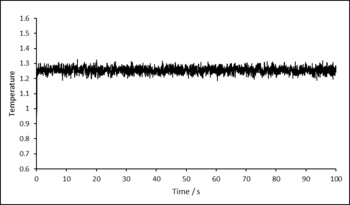
Figure 1: Temperature as a function of time.
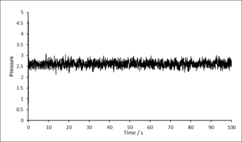
Figure 2: Pressure as a function of time.
Figure 3: Total energy as a function of time.

5 time-steps were tested to determine the most adequate. Figure 4 to the right shows how the total energy changes over time for each of the 5 timesteps. It can be seen that a time-step of 0.0025 is the highest time-step that still gives an accurate equilibrium total energy, hence, this time-step was used in further simulations.

Figure 4: Total energy as a function of time for 5 different timesteps.

Simulations were run to determine the equation of state of the model described above, by calculating the density of a NpT system at varying pressure and temperature. 2 pressures and 5 temperatures were chosen (p = 2.5, 2.75; T = 1.75, 2, 2, 2.25, 3, 5), and a simulation was run for each combination giving a total of 10 phase points.

Simulations were run to determine the change in constant volume heat capacity with temperature. 2 densities and 5 temperatures were chosen ( $ρ$ = 0.2, 0.8; T = 2.0, 2.2, 2.4, 2.6, 2.8), giving a total of 10 phase points.

Simulations were run to model the radial distribution function as a function of distance, using the software VMD. 3 simulations were run, each with a specified density and temperature correlating to a system in each of the 3 phases^[1]: solid, liquid and gas.

Solid: Density = 1.25, Temperature = 1.0
Liquid: Density = 0.8, Temperature = 1.2
Gas: Density = 0.025, Temperature = 1.2

You do not really need to specify VMD here - there are a host of programs that can calculate a RDF, and not so hard a program to write yourself. If you insist on specifying VMD, the full name and citation would be good.

The mean squared displacement (MSD) and velocity autocorrelation function (VACF) were calculated using the same densities and temperatures specified above (same as RDF) to model a system in each of the 3 phases. Both the MSD and VACF were used to calculate the diffusion coefficient (D) for each phase, using the following relationships.

$D = \frac{1}{6} \frac{\partial ⟨ r^{2} (t) ⟩}{\partial t}$

$D = \frac{1}{3} \int_{0}^{\infty} d τ ⟨ v (0) \cdot v (τ) ⟩$

Results & Discussion

Equations of state

Figure 5: Density as a function of temperature for a system at 2 different pressures, as well as the corresponding densities as predicted by the ideal gas law.

For all systems, density decreases with increasing temperature. The simulated density is lower than that predicted by the ideal gas law. This is because the ideal gas law does not take into account all the interactions between particles, whereas the simulation contains information regarding pairwise interactions modelled on the L-J potential. Hence, in the simulation, the atoms are further apart due to these repulsive interactions, and the density is lower.

The discrepancy between the simulated density and the density predicted by the ideal gas law decreases with increasing temperature as the particles have enough energy to overcome the repulsive interactions and move more freely - hence, as temperature increases, the system more closely models an ideal gas.

Scientific style: instead of e.g. "more closely models and ideal gas" perhaps something like "tends toward the ideal gas eq. of state in the high temperature limit. Also an explanation of why this is would be beneficial here - think about what happens in terms of phase space sampling at a given temperature. How could you connect that to the PES and PE/KE a given LJ particle has?

Heat capacity at constant volume

Figure 6: Constant volume heat capacity as a function of temperature for 2 different densities.

The expected trend of heat capacity decreasing with increasing temperature is observed. For this system, the density, number of particles and total energy remain constant. Furthermore, the total energy of the system at equilibrium is equal for every run. Hence, by analysing the below equation:

$C_{V} = N^{2} \frac{⟨ E^{2} ⟩ - {⟨ E ⟩}^{2}}{k_{B} T^{2}}$

It is evident that with increasing temperature, constant volume heat capacity decreases.

The heat capacity also increases with increasing density, this is due to there being more atoms and hence more energy states that need to be populated. Therefore, it requires a higher temperature to fill the states and increase the total energy of the system.

Radial distribution function

The RDF for the gas shows one peak corresponding to the single coordination shell of the central particle. The RDF then decays to a value of 1, this is because outside of the primary coordination shell, the particles are very diffuse with no order.

The RDF for the liquid shows 4 peaks of decreasing intensity corresponding to coordination shells of increasing radius around the central particle. The decrease in intensity is due to the decrease in order of the particles in the shells as distance increases. As distance increases this order further decreases as particles are more free to move causing the RDF to decay to the bulk density value.

The RDF for the solid shows multiple peaks of varying intensity. This is due to the fact that the solid is based on a crystal structure with a regular repeated and fixed structure. Again, the peaks coordinate to coordination shells around the central particle. In a solid therefore, there is always long range order.

A more quantitative discussion would be good.

Diffusion coefficient

MSD Method

Plots displaying the mean squared displacement as a function of time-step are below:

Figure 8: Mean squared displacement as a function of timestep for a system in the gas phase.
Figure 9: Mean squared displacement as a function of timestep for a system in the liquid phase.
Figure 10: Mean squared displacement as a function of timestep for a system in the solid phase.

Plots displaying the mean squared displacement as a function of time-step for a system with 1,000,000 atoms are below:

Figure 11: Mean squared displacement as a function of timestep for a system in the gas phase for a system of 1,000,000 atoms.
Figure 12: Mean squared displacement as a function of timestep for a system in the liquid phase for a system of 1,000,000 atoms.
Figure 13: Mean squared displacement as a function of timestep for a system in the solid phase for a system of 1,000,000 atoms.

The diffusion coefficient for each system was calculated by measuring the gradient of the flat region of each graph. The values for each system are below:

Figure 14: Diffusion coefficient values calculated from MSD method.

First, analysing the mean squared displacement graphs, all graphs display the expected trends. For a solid, atoms are fixed in position and therefore the gradient is close to 0 as they do not deviate from their original positions. The fluctuations in the original simulation (Figure 10) are caused by atoms vibrating, resulting in small deviations away from their starting positions.

For both liquid and gas, the expected trends of MSD increasing with time are shown. As both liquid and gas particles are able to diffuse through the system, over time they diffuse further away from their starting position. For gas, the increase in MSD is much faster than for the liquid as the gas particles are able to diffuse much easier, due to the fact that in a gas the particles are much more diffuse allowing them to move more freely through the system, without interacting with other particles.

The diffusion coefficients are as expected with that of the gas being much larger than for the liquid and the solid, due to the gaseous system being much more diffuse. With the diffusion coefficient of the solid being close to 0, as the atoms are fixed and therefore cannot deviate from their original position. For the liquid system, there is some short range order however particles are able to move away from their starting position, though due to the much higher density than the gas, there are interactions between particles which increase the amount of time in which it takes them to move away.

The data from the original simulation is very similar to that of the 1,000,000 atom simulation though it is to be expected that the 1,000,000 atom simulation is much more accurate as it is a larger system and therefore more data contributes to the average. A discussion of finite size effects - even if not a systematic investigation - would have been nice here. VACF Method

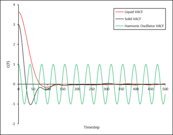
Figure 15: VACF as a function of time for the solid and liquid phases along with the 1D Harmonic oscillator.
Figure 16: Running integral of the VACF for the original simulation.
Figure 17: Running integral of the VACF for the 1,000,000 atom simulation.

The trapezium rule was used to calculate the integral of the VACF for each phase.

The diffusion coefficients were then calculated from the total integral using the relationship stated in the introduction, the calculated values are displayed below in Figure 18.

Note: For the gas phase in the initial simulation, the running integral does not converge on one maximum value, the diffusion coefficient could not be accurately calculated.

In the VACF as a function of time plot (Figure 15), the maxima and minima of the solid and liquid functions correspond to the change in velocity of a particle after a collision. However, the VACF of the liquid decays much faster due to the more diffuse nature of the liquid allowing particles to diffuse away from each other, something that is not possible in a solid due to the fixed positions of the atoms.

The VACF for the harmonic oscillator does not dampen as the model assumes that particles do not lose energy, furthermore the model does not take into account key interactions between particles (which the simulation does) for example the interactions of the Leonard-Jones system.

Again the diffusion coefficients are as expected, with that of the gas being much larger than for liquid and solid, and the solid diffusion coefficient being close to 0. Furthermore, the values compare well to those calculated using the MSD method. There is again similarity between the original simulation and 1,000,000 atom simulation however it is expected that the 1,000,000 atom simulation is more accurate due to more data contributing to the average. The largest source of error in the estimates of D (from the VACF method) comes from the error in using the trapezium rule.

Conclusion

Equation of state simulations, on a system of constant pressure determined that the density of a system at constant pressure decreased with increasing temperature. The simulated density is lower than that predicted by the ideal gas law as the system is not behaving ideally (there are interactions between the particles), however this discrepancy decreases with increasing temperature.

Heat capacity simulations showed the expected trend of heat capacity at constant volume decreasing with increasing temperature. Furthermore, heat capacity increases with increasing density as there are more particles and hence more energy states that need to be filled to increase the temperature, therefore requiring a larger amount of energy to do so.

Radial distribution function simulations gave information about the coordination around particles in each phase. The solid has a regular ordered crystal structure and hence the radial distribution function displays many peaks. For liquids there is some short range order, shown by 4 peaks of decreasing intensity corresponding to 4 initial coordination shells around the liquid, however it decays quickly due to the ability of particles to diffuse away, resulting in very little long range order. For a gas, there is one initial coordination shell shown by the sharp initial peak, however it then decays to the bulk density value and remains constant due to the high diffusive nature of a gas, there is no long range order past this first coordination shell.

Both methods of calculation of the diffusion coefficient give the expected results, with a gas having a large value, liquid a small value and the solid with a value close to 0. The values obtained from each method compare well to each other, as well as the values obtained from the 1,000,000 atom simulation. However, it is expected that the 1,000,000 atom simulation is more accurate due to more data contributing to the average. Furthermore, the VACF method will have significant error due to the error in using the trapezium rule to calculate the integral of the VACF.

In conclusion, molecular dynamics simulation has allowed fast and accurate how are you measuring accuracy. You would need to fit LJ parameters for a specific system, then compare to experiment or a higher accuracy simulation/theory. calculations of a range of key thermodynamic properties of a range of systems. It is clear that the use of these simulations is invaluable for the determination of these properties with applications in a range of industries, on key example being in the design of power stations. Furthermore, none of the simulations took longer than 5 minutes How long is a piece of string? Yes they are very cheap, but you cannot specify a time without giving the length of the simulations exactly, software package details (you did this), computer architecture etc. , illustrating another key benefit of using molecular dynamics simulations. In future calculations, calculations should be done on larger systems to acquire a more accurate average, as well as possibly introducing a second type of particle into the system to analyse how it effects the properties of the system. Nice that you've attempted a small outlook. Perhaps think about the LJ model itself. Would you want to keep using larger and larger LJ systems. Would you want to use specific LJ parameters next time for a specific system? Or perhaps a different force field?

Tasks

The answers to all tasks are below, some have already been answered in the report above.

Introduction to molecular dynamics simulation

TASK: Open the file HO.xls. In it, the velocity-Verlet algorithm is used to model the behaviour of a classical harmonic oscillator. Complete the three columns "ANALYTICAL", "ERROR", and "ENERGY": "ANALYTICAL" should contain the value of the classical solution for the position at time $t$ , "ERROR" should contain the absolute difference between "ANALYTICAL" and the velocity-Verlet solution (i.e. ERROR should always be positive -- make sure you leave the half step rows blank!), and "ENERGY" should contain the total energy of the oscillator for the velocity-Verlet solution. Remember that the position of a classical harmonic oscillator is given by $x (t) = A \cos (ω t + ϕ)$ (the values of $A$ , $ω$ , and $ϕ$ are worked out for you in the sheet).

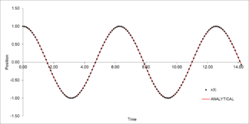
Figure 19: Analytical position as a function of time for the harmonic oscillator
Figure 20: Total energy as a function time for the harmonic oscillator
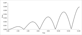
Figure 21: Error between the velocity-Verlet algorithm and analytical values as a function of time for the harmonic oscillator

TASK: For the default timestep value, 0.1, estimate the positions of the maxima in the ERROR column as a function of time. Make a plot showing these values as a function of time, and fit an appropriate function to the data.

Figure 22: Error maximum as a function of time for the harmonic oscillator

required time step for HO missing.

TASK: For a single Lennard-Jones interaction, $ϕ (r) = 4 ϵ (\frac{σ^{12}}{r^{12}} - \frac{σ^{6}}{r^{6}})$ , find the separation, $r_{0}$ , at which the potential energy is zero. What is the force at this separation? Find the equilibrium separation, $r_{e q}$ , and work out the well depth ( $ϕ (r_{e q})$ ). Evaluate the integrals $\int_{2 σ}^{\infty} ϕ (r) d r$ , $\int_{2.5 σ}^{\infty} ϕ (r) d r$ , and $\int_{3 σ}^{\infty} ϕ (r) d r$ when $σ = ϵ = 1.0$ .

The separation r₀ at which the potential energy is zero, is when $r$ ₀ $= σ$
The force at this separation is equal to $24 ϵ / σ$
The equilibrium separation $r$ _eq $= 2$ ^1/6 $σ$
The potential well depth is equal to $- ϵ$
Evaluation of integrals:

TASK: Estimate the number of water molecules in 1ml of water under standard conditions. Estimate the volume of $10000$ water molecules under standard conditions.

Assumptions:

1mL of water = 1g of water

Number of water molecules in 1g:

Moles in 1g = 1/18
Number of molecules = N_A x 1/18 = 3.35 x10²²

Volume of 10000 water molecules:

Moles = 10000/N_A = 1.66 x10^-20
Mass = 1.66 x10^-20 x 18 = 2.99 x10^-19g
Volume = 2.99 x10^-19mL

TASK: Consider an atom at position $(0.5, 0.5, 0.5)$ in a cubic simulation box which runs from $(0, 0, 0)$ to $(1, 1, 1)$ . In a single timestep, it moves along the vector $(0.7, 0.6, 0.2)$ . At what point does it end up, after the periodic boundary conditions have been applied?.

It ends up at the point with coordinates - $(0.2, 0.1, 0.7)$

TASK: The Lennard-Jones parameters for argon are $σ = 0.34 n m, ϵ / k_{B} = 120 K$ . If the LJ cutoff is $r^{*} = 3.2$ , what is it in real units? What is the well depth in ${k J m o l}^{- 1}$ ? What is the reduced temperature $T^{*} = 1.5$ in real units?

LJ cutoff in real units $= 1.088 n m$
Well Depth $= 0.998 k J m o l$ ^-1
Reduced Temperature $= 180 K$

Equilibration

TASK: Why do you think giving atoms random starting coordinates causes problems in simulations? Hint: what happens if two atoms happen to be generated close together?

Atoms cannot be given random starting coordinates as there is a high chance of atoms being generated close to each other resulting in an unnatural interaction (repulsion) between the two. Yes. but why is this a bad things in terms of the simulation? Under what simulation parameters would the system equilibrate correctly anyway?

TASK: Satisfy yourself that this lattice spacing corresponds to a number density of lattice points of $0.8$ . Consider instead a face-centred cubic lattice with a lattice point number density of 1.2. What is the side length of the cubic unit cell?

For a face-centred cubic lattice with a lattice point density of 1.2, the side length of the cubic unit cell is 1.494.

TASK: Consider again the face-centred cubic lattice from the previous task. How many atoms would be created by the create_atoms command if you had defined that lattice instead?

A face-centred cubic lattice has 4 lattice points and hence four atoms, whereas a cubic lattice has 1 of each. Therefore, there would be 4000 atoms in a 10 x 10 x 10 box.

TASK: Using the LAMMPS manual, find the purpose of the following commands in the input script:

mass 1 1.0
pair_style lj/cut 3.0
pair_coeff * * 1.0 1.0

Line 1: Sets the mass of all atoms of type 1 to 1.0
Line 2: States that the interaction between atoms is to be modelled on the Leonard-Jones potential with a cut off distance of 3.0
Line 3: Sets the pairwise force field coefficients for all atoms, in this case, this is the well depth and the distance at 0 potential - both are set to 1.0

TASK: Given that we are specifying $x_{i} (0)$ and $v_{i} (0)$ , which integration algorithm are we going to use?

The Velocity-Verlet Algorithm.

TASK: Look at the lines below.

### SPECIFY TIMESTEP ###
variable timestep equal 0.001
variable n_steps equal floor(100/${timestep})
timestep ${timestep}

### RUN SIMULATION ###
run ${n_steps}
run 100000

The second line (starting "variable timestep...") tells LAMMPS that if it encounters the text ${timestep} on a subsequent line, it should replace it by the value given. In this case, the value ${timestep} is always replaced by 0.001. In light of this, what do you think the purpose of these lines is? Why not just write:

timestep 0.001
run 100000

The initial script sets the time-step as a variable which can be called later in the script, the second script does not do this. Therefore, if a simulation is to be run on a different time-step, the input file with the initial script only needs to change the time-step in one place (where the variable is defined). Whereas, in the second script, the time-step will have to be changed everywhere that it is used in the input file.

TASK: make plots of the energy, temperature, and pressure, against time for the 0.001 timestep experiment (attach a picture to your report). Does the simulation reach equilibrium? How long does this take? When you have done this, make a single plot which shows the energy versus time for all of the timesteps (again, attach a picture to your report). Choosing a timestep is a balancing act: the shorter the timestep, the more accurately the results of your simulation will reflect the physical reality; short timesteps, however, mean that the same number of simulation steps cover a shorter amount of actual time, and this is very unhelpful if the process you want to study requires observation over a long time. Of the five timesteps that you used, which is the largest to give acceptable results? Which one of the five is a particularly bad choice? Why?

Figure 23: Temperature as a function of time for a timestep of 0.001.
Figure 24: Pressure as a function of time for a timestep of 0.001.
Figure 25: Total energy as a function of time for a timestep of 0.001.

It takes approximately 0.3s for the system to reach equilibrium. seconds? I thought we were in LJ units.

Figure 26: Total energy as a function of time for 5 different timesteps.

Of the 5 timesteps, 0.0025 is the largest to give acceptable results. A timestep of 0.015 is particularly bad as the system does not reach equilibrium at all. The other 4 time steps do all reach equilibrium however 0.001 and 0.0025 are the only two which reach an accurate equilibrium value for total energy.

Running simulations under specific conditions

TASK: Choose 5 temperatures (above the critical temperature $T^{*} = 1.5$ ), and two pressures (you can get a good idea of what a reasonable pressure is in Lennard-Jones units by looking at the average pressure of your simulations from the last section). This gives ten phase points — five temperatures at each pressure. Create 10 copies of npt.in, and modify each to run a simulation at one of your chosen $(p, T)$ points. You should be able to use the results of the previous section to choose a timestep. Submit these ten jobs to the HPC portal. While you wait for them to finish, you should read the next section.

TASK: We need to choose $γ$ so that the temperature is correct $T = 𝔗$ if we multiply every velocity $γ$ . We can write two equations:

$\frac{1}{2} \sum_{i} m_{i} v_{i}^{2} = \frac{3}{2} N k_{B} T$

$\frac{1}{2} \sum_{i} m_{i} {(γ v_{i})}^{2} = \frac{3}{2} N k_{B} 𝔗$

Solve these to determine $γ$ .

TASK: Use the manual page to find out the importance of the three numbers 100 1000 100000. How often will values of the temperature, etc., be sampled for the average? How many measurements contribute to the average? Looking to the following line, how much time will you simulate?

The three numbers correspond Nevery, Nrepeat and Nfreq.

Nevery corresponds to how often input values are sampled for the average - for example, temperature will be sampled for the average every 100 timesteps.
Nrepeat corresponds to the number of values used to calculate the average - in this case 1000 values (measurements) are used (contribute) to calculating the average.
Nfreq corresponds to the timestep at which the average is calculated - the 100000th timestep.

This therefore means that there are 100000 timesteps and with a timestep of 0.0025, the time simulated = 250 seconds.

TASK: When your simulations have finished, download the log files as before. At the end of the log file, LAMMPS will output the values and errors for the pressure, temperature, and density $(\frac{N}{V})$ . Use software of your choice to plot the density as a function of temperature for both of the pressures that you simulated. Your graph(s) should include error bars in both the x and y directions. You should also include a line corresponding to the density predicted by the ideal gas law at that pressure. Is your simulated density lower or higher? Justify this. Does the discrepancy increase or decrease with pressure?

Figure 28: Density as a function of temperature for a system at 2 different pressures.

For all systems, density decreases with increasing temperature. The simulated density is lower than that predicted by the ideal gas law. This is because the ideal gas law does not take into account all the interactions between particles, whereas the simulation contains information regarding pairwise interactions modelled on the L-J potential. Hence, in the simulation, the atoms are further apart due to these repulsive interactions, and the density is lower.

The discrepancy between the simulated density and the density predicted by the ideal gas law decreases with increasing temperature as the particles have enough energy to overcome the repulsive interactions and move more freely - hence, as temperature increases, the system more closely models an ideal gas.

Calculating heat capacities using statistical physics

TASK: As in the last section, you need to run simulations at ten phase points. In this section, we will be in density-temperature $(ρ^{*}, T^{*})$ phase space, rather than pressure-temperature phase space. The two densities required at $0.2$ and $0.8$ , and the temperature range is $2.0, 2.2, 2.4, 2.6, 2.8$ . Plot $C_{V} / V$ as a function of temperature, where $V$ is the volume of the simulation cell, for both of your densities (on the same graph). Is the trend the one you would expect? Attach an example of one of your input scripts to your report.

Figure 29: Constant volume heat capacity as a function of temperature.

The expected trend of heat capacity decreasing with increasing temperature is observed. For this system, the density, number of particles and total energy remain constant. Furthermore, the total energy of the system at equilibrium is equal for every run. Hence, by analysing the below equation:

$C_{V} = N^{2} \frac{⟨ E^{2} ⟩ - {⟨ E ⟩}^{2}}{k_{B} T^{2}}$

It is evident that with increasing temperature, constant volume heat capacity decreases.

The heat capacity also increases with increasing density, this is due to there being more atoms and hence more energy states that need to be populated. Therefore, it requires a higher temperature to fill the states and increase the total energy of the system.

An example of the input script used can be found below:

File:ExampleInputFileJPW.in

Structural properties and the radial distribution function

TASK: perform simulations of the Lennard-Jones system in the three phases. When each is complete, download the trajectory and calculate $g (r)$ and $\int g (r) d r$ . Plot the RDFs for the three systems on the same axes, and attach a copy to your report. Discuss qualitatively the differences between the three RDFs, and what this tells you about the structure of the system in each phase. In the solid case, illustrate which lattice sites the first three peaks correspond to. What is the lattice spacing? What is the coordination number for each of the first three peaks?

The RDF for the gas shows one peak corresponding to the single coordination shell of the central particle. The RDF then decays to a value of 1, this is because outside of the primary coordination shell, the particles are very diffuse and therefore the chance of finding another particle is equal to the bulk density value.

The RDF for the liquid shows 4 peaks of decreasing intensity corresponding to coordination shells of increasing radius around the central particle. The decrease in intensity is due to the decrease in order of the particles in the shells as distance increases. As distance increases this order further decreases as particles are more free to move causing the RDF to decay to the bulk density value.

The RDF for the solid shows multiple peaks of varying intensity. This is due to the fact that the solid is based on a crystal structure with a regular repeated and fixed structure. Again, the peaks coordinate to coordination shells around the central particle. In a solid therefore, there is always long range order.

You did not answer the some of the question: In the solid case, illustrate which lattice sites the first three peaks correspond to. What is the lattice spacing? What is the coordination number for each of the first three peaks?.

Dynamic properties and the diffusion coefficient

TASK: In the D subfolder, there is a file liq.in that will run a simulation at specified density and temperature to calculate the mean squared displacement and velocity autocorrelation function of your system. Run one of these simulations for a vapour, liquid, and solid. You have also been given some simulated data from much larger systems (approximately one million atoms). You will need these files later.

TASK: make a plot for each of your simulations (solid, liquid, and gas), showing the mean squared displacement (the "total" MSD) as a function of timestep. Are these as you would expect? Estimate $D$ in each case. Be careful with the units! Repeat this procedure for the MSD data that you were given from the one million atom simulations.

Figure 30: Mean squared displacement as a function of timestep for a system in the gas phase.
Figure 31: Mean squared displacement as a function of timestep for a system in the liquid phase.
Figure 32: Mean squared displacement as a function of timestep for a system in the solid phase.

Figure 33: Mean squared displacement as a function of timestep for a system in the gas phase for a system of 1,000,000 atoms.
Figure 34: Mean squared displacement as a function of timestep for a system in the liquid phase for a system of 1,000,000 atoms.
Figure 35: Mean squared displacement as a function of timestep for a system in the solid phase for a system of 1,000,000 atoms.

The diffusion coefficient for each system was calculated by measuring the gradient of the flat region of each graph. The values for each system are below:

Figure 36: Diffusion coefficient values calculated from MSD method.

First, analysing the mean squared displacement graphs, all graphs display the expected trends. For a solid, atoms are fixed in position and therefore the gradient is close to 0 as they do not deviate from their original positions. The fluctuations in the original simulation (Figure X) are caused by atoms vibrating, resulting in small deviations away from their starting positions.

For both liquid and gas, the expected trends of MSD increasing with time are shown. As both liquid and gas particles are able to diffuse through the system, over time they diffuse further away from their starting position. For gas, the increase in MSD is much faster than for the liquid as the gas particles are able to diffuse much easier, due to the fact that in a gas the particles are much more diffuse allowing them to move more freely through the system, without interacting with other particles.

The diffusion coefficients are as expected with that of the gas being much larger than for the liquid and the solid, due to the gaseous system being much more diffuse. With the diffusion coefficient of the solid being close to 0, as the atoms are fixed and therefore cannot deviate from their original position. For the liquid system, there is some short range order however particles are able to move away from their starting position, though due to the much higher density than the gas, there are interactions between particles which increase the amount of time in which it takes them to move away.

The data from the original simulation is very similar to that of the 1,000,000 atom simulation though it is to be expected that the 1,000,000 atom simulation is much more accurate as it is a larger system and therefore more data contributes to the average.

TASK: In the theoretical section at the beginning, the equation for the evolution of the position of a 1D harmonic oscillator as a function of time was given. Using this, evaluate the normalised velocity autocorrelation function for a 1D harmonic oscillator (it is analytic!):

$C (τ) = \frac{\int_{- \infty}^{\infty} v (t) v (t + τ) d t}{\int_{- \infty}^{\infty} v^{2} (t) d t}$

Be sure to show your working in your writeup. On the same graph, with x range 0 to 500, plot $C (τ)$ with $ω = 1 / 2 π$ and the VACFs from your liquid and solid simulations. What do the minima in the VACFs for the liquid and solid system represent? Discuss the origin of the differences between the liquid and solid VACFs. The harmonic oscillator VACF is very different to the Lennard Jones solid and liquid. Why is this? Attach a copy of your plot to your writeup.

The derivation for the normalised velocity autocorrelation function for a 1D harmonic oscillator is shown below, along with two trigonometric identities used in the derivation.

Figure 37: Trigonometric identities used in derivation of VACF of 1D Harmonic Oscillator

Figure 38: Derivation of the VACF of 1D Harmonic Oscillator

A plot showing the VACF for the liquid and solid simulations, as well as for a 1D harmonic oscillator with $ω = 1 / 2 π$ is shown below:

Figure 39: VACF as a function of timestep for the liquid and solid phases as well as for a 1D harmonic oscillator.

In the VACF as a function of time plot (Figure 39), the maxima and minima of the solid and liquid functions correspond to the change in velocity of a particle after a collision. However, the VACF of the liquid decays much faster due to the more diffuse nature of the liquid allowing particles to diffuse away from each other, something that is not possible in a solid due to the fixed positions of the atoms.

The VACF for the harmonic oscillator does not dampen as the model assumes that particles do not lose energy, furthermore the model does not take into account key interactions between particles (which the simulation does) for example the interactions of the Leonard-Jones system.

TASK: Use the trapezium rule to approximate the integral under the velocity autocorrelation function for the solid, liquid, and gas, and use these values to estimate $D$ in each case. You should make a plot of the running integral in each case. Are they as you expect? Repeat this procedure for the VACF data that you were given from the one million atom simulations. What do you think is the largest source of error in your estimates of D from the VACF?

Figure 40: Running integral of the VACF for the original simulation.
Figure 41: Running integral of the VACF for the 1,000,000 atom simulation.

The diffusion coefficients were calculated from the total integral using the relationship stated in the introduction, the calculated values are displayed below in Figure X.

Note: For the gas phase in the initial simulation, the running integral does not converge on one maximum value, the diffusion coefficient could not be accurately calculated.

Again the diffusion coefficients are as expected, with that of the gas being much larger than for liquid and solid, and the solid diffusion coefficient being close to 0. Furthermore, the values compare well to those calculated using the MSD method. There is again similarity between the original simulation and 1,000,000 atom simulation however it is expected that the 1,000,000 atom simulation is more accurate due to more data contributing to the average. The largest source of error in the estimates of D (from the VACF method) comes from the error in using the trapezium rule.

References

↑ J.P.Hansen, L.Verlet, Phys.Rev., 1969, 184, 151

[L-J_Article-1] J.P.Hansen, L.Verlet, Phys.Rev., 1969, 184, 151

[1]