Talk:Yc9014-liquid

JC: General comments: All tasks answered, but explanations lacked a lot of detail. Try to write a few sentences to explain the significance of your results and demonstrate that you understand the underlying theory behind the steps in the experiment.

part 2:Introduction to molecular dynamics simulation

TASK: For the default timestep value, 0.1, estimate the positions of the maxima in the ERROR column as a function of time. Make a plot showing these values as a function of time, and fit an appropriate function to the data.

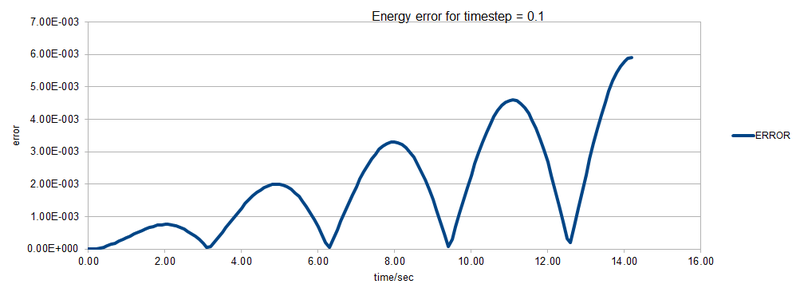
JC: Why does the error oscillate?

TASK: Experiment with different values of the timestep. What sort of a timestep do you need to use to ensure that the total energy does not change by more than 1% over the course of your "simulation"? Why do you think it is important to monitor the total energy of a physical system when modelling its behaviour numerically?

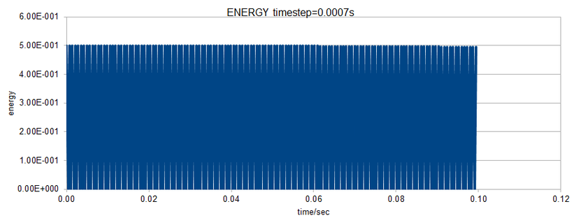
To ensure total energy change within 1%, we need at most 0.0007s as our time step. We assume that the total energy is a constant for this physical model, however it is not steady in reality, so me need to monitor the total energy to make sure the difference in total energy is within a acceptable range.

JC: The graph shows a change in energy of 100%, it looks like you're only showing the potential or kinetic energy, but not the total energy.

TASK: Lennard-Jones interaction

Find the separation, and at which the potential energy is zero. What is the force at this separation?

For a single Lennard-Jones interaction,$\varphi \left(r\right)=4ϵ(\frac{{\sigma }^{12}}{r^{12}}-\frac{{\sigma }^6}{r^6})$, when potential energy is zero,

$0=4ϵ(\frac{{\sigma }^{12}}{r^{12}}-\frac{{\sigma }^6}{r^6})$

$\frac{{\sigma }^{12}}{r^{12}}=\frac{{\sigma }^6}{r^6}$

Distance r is a positive value , so r=σ,

Force at this separation, $F=-\frac{\mathrm{d}U\left({\mathbf{r}}^N\right)}{\mathrm{d}{\mathbf{r}}_i}=-4ϵ(\frac{-12{\sigma }^{12}}{r^{13}}+6\frac{{\sigma }^6}{r^7})=-4ϵ(\frac{-12}{\sigma }+\frac{6}{\sigma })=\frac{-24ϵ}{\sigma }$

Find the equilibrium separation, and work out the well depth $\varphi \left(r_{eq}\right)$ At equilibrium separation, F=0

$F=-4ϵ(\frac{-12{\sigma }^{12}}{r^{13}}+6\frac{{\sigma }^6}{r^7})=0$

$\frac{2{\sigma }^6}{r^6}=1$

$r=2^{1/6}\sigma$,

$\varphi \left(r_{eq}\right)=4ϵ(\frac{{\sigma }^{12}}{r^{12}}-\frac{{\sigma }^6}{r^6})=4ϵ(\frac{{\sigma }^{12}}{(2^{\frac{1}{6}}r{)}^{12}}-\frac{{\sigma }^6}{(2^{\frac{1}{6}}r{)}^6})=4ϵ(\frac{{\sigma }^{12}}{4r^{12}}-\frac{{\sigma }^6}{2r^6})=4ϵ(\frac{1}{4}-\frac{1}{2})=-ϵ$

Evaluate the integrals $\underset{2\sigma }{\overset{\mathrm{\infty }}{\int }}\varphi \left(r\right)\mathrm{d}r$, $\underset{2.5\sigma }{\overset{\mathrm{\infty }}{\int }}\varphi \left(r\right)\mathrm{d}r$, and $\underset{3\sigma }{\overset{\mathrm{\infty }}{\int }}\varphi \left(r\right)\mathrm{d}r$ when $\sigma =ϵ=1.0$.

$\underset{2\sigma }{\overset{\mathrm{\infty }}{\int }}\varphi \left(r\right)\mathrm{d}r=4ϵ\underset{2\sigma }{\overset{\mathrm{\infty }}{\int }}(\frac{-{\sigma }^{12}}{11r^{11}}+\frac{{\sigma }^6}{5r^5})=0-4ϵ(\frac{-{\sigma }^{12}}{11\times 2.5^{11}\times {\sigma }^{11}}+\frac{{\sigma }^6}{5\times 2.5^5\times {\sigma }^5})=-2.48\times 10^{-2}$

$\underset{2.5\sigma }{\overset{\mathrm{\infty }}{\int }}\varphi \left(r\right)\mathrm{d}r=4ϵ\underset{2.5\sigma }{\overset{\mathrm{\infty }}{\int }}(\frac{-{\sigma }^{12}}{11r^{11}}+\frac{{\sigma }^6}{5r^5})=0-4ϵ(\frac{-{\sigma }^{12}}{11\times 2^{11}\times {\sigma }^{11}}+\frac{{\sigma }^6}{5\times 2^5\times {\sigma }^5})=-8.18\times 10^{-3}$

$\underset{3\sigma }{\overset{\mathrm{\infty }}{\int }}\varphi \left(r\right)\mathrm{d}r=4ϵ\underset{3\sigma }{\overset{\mathrm{\infty }}{\int }}(\frac{-{\sigma }^{12}}{11r^{11}}+\frac{{\sigma }^6}{5r^5})=0-4ϵ(\frac{-{\sigma }^{12}}{11\times 3^{11}\times {\sigma }^{11}}+\frac{{\sigma }^6}{5\times 3^5\times {\sigma }^5})=-3.29\times 10^{-3}$

JC: Correct.

TASK: Estimate the number of water molecules in 1ml of water under standard conditions. Estimate the volume of 10000 water molecules under standard conditions.

Estimate the number of water molecules in 1ml of water under standard conditions.

$n=m/M=\frac{1g}{18g/mol}=\frac{1}{18}mol$

$N=A\times n=6.02*10^{23}/mol\times \frac{1}{18}mol=3.34\times 10^{-19}$

Estimate the volume of 10000 water molecules under standard conditions

$\frac{18mL}{A}\times 10000=2.99\times 10^{-19}mL$

TASK: Consider an atom at position $(0.5,0.5,0.5)$ in a cubic simulation box which runs from $(0,0,0)$ to $(1,1,1)$. In a single timestep, it moves along the vector $(0.7,0.6,0.2)$. At what point does it end up, after the periodic boundary conditions have been applied?

(0.2,0.1,0.7)

TASK: The Lennard-Jones parameters for argon are $\sigma =0.34\mathrm{n}\mathrm{m}$, $$\begin{gathered} ϵ \\ / \\ {k}_B=120\mathrm{K} \end{gathered}$$. If the LJ cutoff is $r^{*}=3.2$, what is it in real units? What is the well depth in $$\begin{gathered} {\mathrm{k}\mathrm{J} \\ \mathrm{m}\mathrm{o}\mathrm{l}}^{-1} \end{gathered}$$? What is the reduced temperature $T^{*}=1.5$ in real units?

r=r*$\times$σ=3.2 $\times$ 0.34nm=1.088 nm

ε=120k$\times$ kb=$120K\times 1.38\times 10^{-23}J/K$=$1.65\times 10^{-21}J=1.65\times 10^{-24}kJ\times 6.02\times 10^{23}/mol=0.9974kJ/mol$

T=T*$\frac{ϵ}{kb}=1.5\times 120K=180K$

JC: Correct.

part 3 : Equilibrium

TASK: Why do you think giving atoms random starting coordinates causes problems in simulations? Hint: what happens if two atoms happen to be generated close together?

They overlap in space, which cannot happen in real life.

JC: The high repulsive forces between atoms can make the simulation unstable and cause it to crash.

TASK: Satisfy yourself that this lattice spacing corresponds to a number density of lattice points of 0.8. Consider instead a face-centred cubic lattice with a lattice point number density of 1.2. What is the side length of the cubic unit cell?

Side length=$(\frac{4}{1.2}{)}^{\frac{1}{3}}=1.4938$

TASK: Consider again the face-centred cubic lattice from the previous task. How many atoms would be created by the create_atoms command if you had defined that lattice instead?

4000

Simple cubic lattice has 1 atom/lattice point per unit cell, face centered cubic lattice has 4 atoms/lattice points per unit cell, our box contains 10*10*10=1000 unit cells, therefore 4000 atoms are generated.

JC: Correct.

TASK: Using the LAMMPS manual, find the purpose of the following commands in the input script:

mass 1 1.0
pair_style lj/cut 3.0
pair_coeff * * 1.0 1.0

For type I atom, mass =1.0 .The lj/cut 3.0 compute the standard 12/6 Lennard-Jones potential while r=3 is the cutoff. Pair_coeff defines the coefficient, in this case, both $ϵ$ and $\sigma$ are 1.

JC: Why is a cut off used with the Lennard-Jones potential?

TASK: Given that we are specifying ${\mathbf{x}}_i\left(0\right)$ and ${\mathbf{v}}_i\left(0\right)$, which integration algorithm are we going to use?

Velocity Verlet algorithm. Classical verlet algorithm cannot make use of ${\mathbf{v}}_i\left(0\right)$ and is less accurate.

what do you think the purpose of these lines is? Why not just write:

timestep 0.001
run 100000

‘timestep 0.001’ only defines a time step at beginning, we need timestep as a varible so that every timestep appears later can be substitute by 0.001.

JC: This is not clear. The point of using a variable is that if the timestep is changed, other commands which depend on the value of the timestep will also be changed automatically.

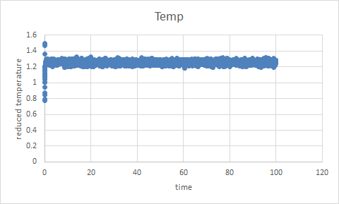
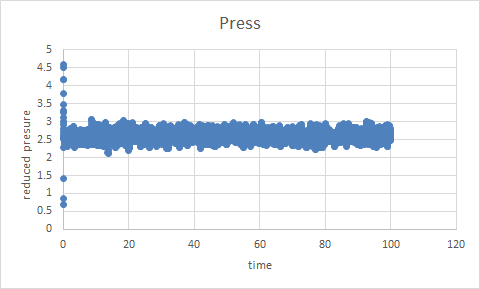
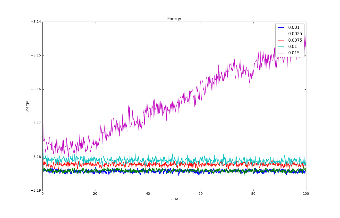
TASK: make plots of the energy, temperature, and pressure, against time for the 0.001 timestep experiment (attach a picture to your report). Does the simulation reach equilibrium? How long does this take? When you have done this, make a single plot which shows the energy versus time for all of the timesteps (again, attach a picture to your report). Choosing a timestep is a balancing act: the shorter the timestep, the more accurately the results of your simulation will reflect the physical reality; short timesteps, however, mean that the same number of simulation steps cover a shorter amount of actual time, and this is very unhelpful if the process you want to study requires observation over a long time. Of the five timesteps that you used, which is the largest to give acceptable results? Which one of the five is a particularly bad choice? Why?

stimulation reaches equilibrium, taking 0.33s.

T=0.01 is the largest acceptable time step, t=0.015 is a bad choice because it does not reach equilibrium.

JC: Should the total energy depend on the timestep? 0.0025 might be a better choice since it gives the same total energy as a smaller timestep.

part 4:Running simulations under specific conditions

TASK: We need to choose $\gamma$ so that the temperature is correct $T=\mathfrak{𝔗}$ if we multiply every velocity $\gamma$. Determine $\gamma$.

$\frac{1}{2}\sum _i{m}_i{v}_i^2=\frac{3}{2}N{k}_{B}T$ equation (1)

$\frac{1}{2}\sum _i{m}_i{\left(\gamma v_i\right)}^2=\frac{3}{2}N{k}_B\mathfrak{𝔗}$ equation (2)

divide two equations (2)/(1)

${\gamma }^2=\frac{T}{\mathfrak{𝔗}}$

$\gamma =(\frac{T}{\mathfrak{𝔗}}{)}^{\frac{1}{2}}$

JC: Correct.

TASK: Use the manual page to find out the importance of the three numbers 100 1000 100000. How often will values of the temperature, etc., be sampled for the average? How many measurements contribute to the average? Looking to the following line, how much time will you simulate?

1 in every 100 time steps is sample for average. 1000 measurements contribute to average. Only simulate once.

JC: What about 100000?

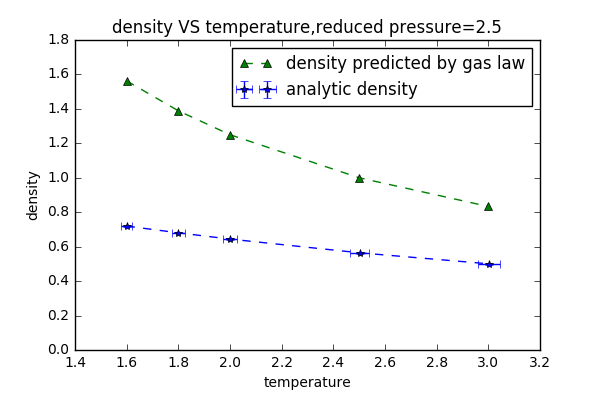
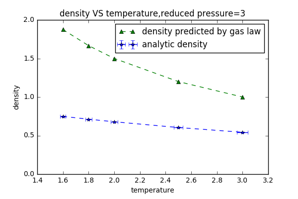
TASK: When your simulations have finished, download the log files as before. At the end of the log file, LAMMPS will output the values and errors for the pressure, temperature, and density \left(\frac{N}{V}\right). Use software of your choice to plot the density as a function of temperature for both of the pressures that you simulated. Your graph(s) should include error bars in both the x and y directions. You should also include a line corresponding to the density predicted by the ideal gas law at that pressure. Is your simulated density lower or higher? Justify this. Does the discrepancy increase or decrease with pressure

Estimated densities are lower than theoretic densities.

The discrepancy increases with the pressure.

JC: Why is this, is this the result you would expect? What are the assumptions made in the ideal gas law which might cause this discrepancy?

paet 5:Calculating heat capacities using statistical physics

TASK: As in the last section, you need to run simulations at ten phase points. In this section, we will be in density-temperature $({\rho }^{*},T^{*})$ phase space, rather than pressure-temperature phase space. The two densities required at 0.2 and 0.8, and the temperature range is 2.0, 2.2, 2.4, 2.6, 2.8. Plot C_V/V as a function of temperature, where V is the volume of the simulation cell, for both of your densities (on the same graph). Is the trend the one you would expect? Attach an example of one of your input scripts to your report.

Script for density= 0.2, temperature=2.0 :File:P=0.2 t=2.txt

Caption

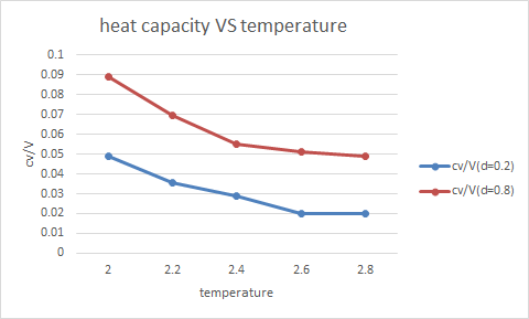
Not expected trend.Heat capacity expected to increase with temperature .

JC: Need to explain this. Why do you expect it to increase with temperature, what about the trend with density?

part 6:Structural properties and the radial distribution function

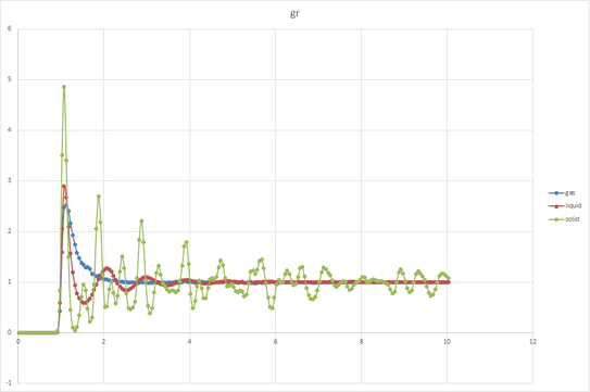
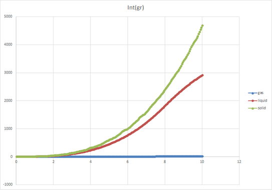
TASK: perform simulations of the Lennard-Jones system in the three phases. When each is complete, download the trajectory and calculate g(r) and $\int g(r)\mathrm{d}r$. Plot the RDFs for the three systems on the same axes, and attach a copy to your report. Discuss qualitatively the differences between the three RDFs, and what this tells you about the structure of the system in each phase. In the solid case, illustrate which lattice sites the first three peaks correspond to. What is the lattice spacing? What is the coordination number for each of the first three peaks?

In graph g(r), we see that gas phase has a very smooth line with only one peak, liquid phase three observable peaks, and solid phase has countless peaks. In lattice model, solid has large density ($N/V)$, so the possibility of finding a neighbor atom(Int(gr)) is larger than liquid and gas. On the contrary, the density of gas is far smaller than both liquid and solid so it has smallest Int(gr). In g(r) graph, solid has many peaks due to its high repeat (lattice) in space, liquid has approximately three smooth observable peaks due to the hydration shells around the particle, gas has only little repeat in long range.

For the nearest neighbors:position would be (0.5,0.5,0)(0,0.5,0.5)(0.5,0,0.5)...12 atoms in total

For the second nearest neighbors:position would be (1,0,0)(-1,0,)(0,1,0)...6 atoms in total

For the third nearest neighbors:position would be (1,1,0)(-1,-1,)(0,1,1)...24 atoms in total

$1.875\sigma =(0.5{)}^{2}r$

$r=2.65\sigma$

JC: Graphs look good, but try to include more detail in your answer. What is the lattice spacing and how did you calculate it?

part 7:Dynamical properties and the diffusion coefficient

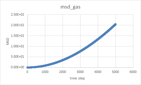
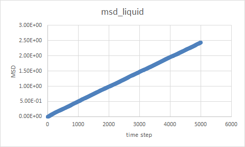
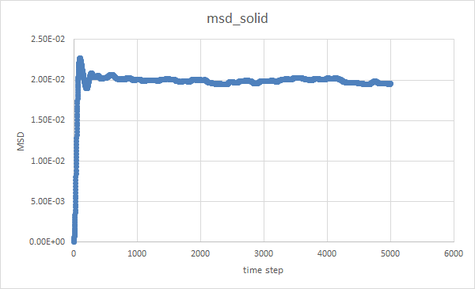
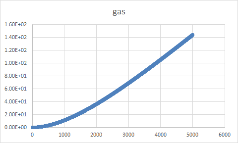
TASK: make a plot for each of your simulations (solid, liquid, and gas), showing the mean squared displacement (the "total" MSD) as a function of timestep. Are these as you would expect? Estimate D in each case. Be careful with the units! Repeat this procedure for the MSD data that you were given from the one million atom simulations.

$D=6\times MSD$

When time step=5000

$D_{(}gas)=204\times 6=1224$

$D_{(}liquid)=2.44\times 6=14.64$

$D_{(}solid)=0.0196\times 6=0.1176$

No unit in the case as all the parameter we use are in their reduced units, however in reality the unit of D would be $distanc{e}^2/time$, for example, $c{m}^2/s$

One million stimulation graphs

JC: Show the lines of best fit on the graphs which were used to calculate the diffusion coefficients, did you fit to the entire data range or just the linear part?

TASK: In the theoretical section at the beginning, the equation for the evolution of the position of a 1D harmonic oscillator as a function of time was given. Using this, evaluate the normalised velocity autocorrelation function for a 1D harmonic oscillator

$C\left(\tau \right)=\frac{\underset{-\mathrm{\infty }}{\overset{\mathrm{\infty }}{\int }}v\left(t\right)v(t+\tau )\mathrm{d}t}{\underset{-\mathrm{\infty }}{\overset{\mathrm{\infty }}{\int }}{v}^2\left(t\right)\mathrm{d}t}$= $=\frac{\underset{-\mathrm{\infty }}{\overset{\mathrm{\infty }}{\int }}\sin (\omega t+\varphi )sin(\omega (t+\tau )+\varphi )\mathrm{d}t}{\underset{-\mathrm{\infty }}{\overset{\mathrm{\infty }}{\int }}{\sin }^2(\omega t+\varphi )\mathrm{d}t}$

For denominator:

Given that $\cos (2x)=1-2{\sin }^{}(x)$

$\underset{-\mathrm{\infty }}{\overset{\mathrm{\infty }}{\int }}{\sin }^2(\omega t+\varphi )\mathrm{d}t=\frac{1}{2}\underset{-\mathrm{\infty }}{\overset{\mathrm{\infty }}{\int }}1-\cos (2\omega t+2\varphi )\mathrm{d}t=\frac{1}{2}[1-\frac{1}{2\omega }\sin (2\omega t+2\varphi ){]}_{-\mathrm{\infty }}^{\mathrm{\infty }}$

For numerator:

Given that $\sin (A+B)=\sin (A)\cos (B)+\cos (A)\sin (B)$

$\underset{-\mathrm{\infty }}{\overset{\mathrm{\infty }}{\int }}\sin (\omega t+\varphi )sin(\omega (t+\tau )+\varphi )\mathrm{d}t=\underset{-\mathrm{\infty }}{\overset{\mathrm{\infty }}{\int }}\sin (\omega t+\varphi )sin(\omega t+\varphi )\cos (\omega \tau )+\sin (\omega t+\varphi )cos(\omega t+\varphi )\sin (\omega \tau )\mathrm{d}t=[\frac{\cos (\omega \tau )}{2}(t-\frac{1}{2\omega }\sin (2\omega t+2\varphi ))+\frac{\sin (\omega \tau )}{2\omega }{\sin }^{}(\omega t+\varphi ){]}_{-\mathrm{\infty }}^{\mathrm{\infty }}$

We know that t is infinity, sin and cos items are negligible compared to t, so

$C\left(\tau \right)=[\frac{\frac{\cos (\omega \tau )}{2}t}{\frac{1}{2}t}{]}_{-\mathrm{\infty }}^{\mathrm{\infty }}=\cos (\omega \tau )$

JC: Correct, but show a few more steps in the working. You can also get this result by splitting the numerator into an integral over sin squared which cancels with the denominator and an integral over sin x cos which is an odd function and so zero.

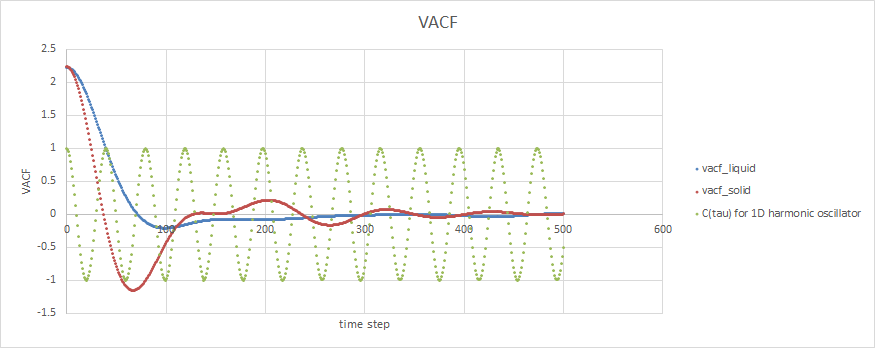
Task: Be sure to show your working in your writeup. On the same graph, with x range 0 to 500, plot $C\left(\tau \right)$ with $\omega =1/2\pi$and the VACFs from your liquid and solid simulations. What do the minima in the VACFs for the liquid and solid system represent? Discuss the origin of the differences between the liquid and solid VACFs. The harmonic oscillator VACF is very different to the Lennard Jones solid and liquid. Why is this? Attach a copy of your plot to your writeup.

Minima in VACF means the state when it has the maximal velocity in the opposite direction, which is when the particle passes the original position. Liquid and solid VACF are different due to different lattice model. Solid has tight lattic point and can only vibrate in a small space and liquid has more degree of free down.

At long range Lennard Jones VACF is approaching 0, but harmonic oscillator VACF still repeats the trigonometric pattern. At long range in Lennard Jones model, the particle does not feel any interaction and so no force apply to the particle therefor the acceleration is 0. However, in harmonic oscillator, the particle repeat simple harmonic oscillation within a certain range, and the VACF is periodic.

JC: The VACF decays to zero due to collisions with other particles which randomises the velocities, there are no collisions in the harmonic oscillator.

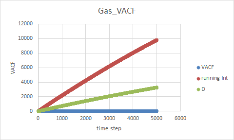
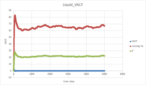
TASK: Use the trapezium rule to approximate the integral under the velocity autocorrelation function for the solid, liquid, and gas, and use these values to estimate D in each case. You should make a plot of the running integral in each case. Are they as you expect? Repeat this procedure for the VACF data that you were given from the one million atom simulations. What do you think is the largest source of error in your estimates of D from the VACF?

As expected, gas has the largest diffusion coefficient and the solid has smallest coefficient. Largest source of error: we assume t is much larger than cos(t) and sin(t) and ignore the trigonometric part, however when t is small, the assumption is no longer doable. There might be a a larger error when t is small.

JC: What about the use of the trapezium rule?