Talk:Wdmn 3rd Year Liquid Simulations

Report

Abstract

Fundamentally, what are you trying to do? We're modelling the dynamics and phase properties of liquids. Say this sort of general stuff here too, not just specifics. Give a purpose for the work.

Molecular dynamic simulations are a well developed technique for probing the qualities of liquids. Here, the temperature dependency of number density and heat capacity was determined for a monoatomic fluid through a Lennard-Jones force field. This gave a comparison between the simulated model and rationalisations from theory. The radial distribution function for a monoatomic solid, liquid and vapour elucidated their different dynamic and structural properties. The diffusion characteristics of each phase was studied from by simulating the mean displacement of an atom from a reference position and the correlation of its future velocities. The results are discussed in relation to the degree of freedom for each phase. The limitation of the model was assessed by simulating with 1000 and 100000 atoms.

Introduction

High-performance computers have made molecular dynamics (MD) simulations a standard lab technique, allowing chemists to probe the behaviour of atoms in extreme reaction conditions. Not just probe the behaviour of atoms in extreme conditions but generally prove the physical properties in dynamic systems. The ability to change thermodynamic parameters such as pressure, temperature and density easily and cheaply has led to its proliferation.

One of the most interesting applications of MD is simulating the conditions found in space. NASA needs to test the stability of metallic alloys and simulates the response of polymeric adhesives in the presence of moisture by MD . Additionally, due to the vast temperature differences between the inside and outside of a spacecraft, being able to assess the thermodynamic properties of electrical conductors is essential for heat management . MD can also be used to determine flow rates, ratios and temperatures for mixing rocket fuel (liquid hydrogen and liquid oxygen). Tick, interesting

Whilst MD simulations have aided the development of new technologies, it has also informed on earth's most abundant and yet enigmatic liquid: water. The evolution of modelling water has progressed from the pairwise force fields implemented in this report to considering many body and quantum effects .

Due to the ability of water to form four strong hydrogen bonds per molecule, which are constantly being broken and reformed because of water's dynamic nature, it displays many anomalous features. Water reaches its most dense state at 4 ^oC and displays extraordinarily high surface tension and low compressibility . This is a result of the competing structural effects of ordered hydrogen bonded tetrahedrons minimising lone pair repulsions at low temperatures and molecules with disordered thermal motion at high temperatures. Water's high polarity gives it an affinity for charged surfaces and makes it the ubiquitous ionic solvent. Water also heavily influences the dynamic and reaction characteristics of proteins. Hydrophobic interactions with carbon chains and hydrogen bonding with permanent dipoles are the driving force for protein folding . Furthermore, the phase diagram water at low temperature and pressure has attracted much attention for its complexity and the presence of a liquid-liquid critical point . Tick

Model and Methodology

Nice methodology

Simulations were performed in LAMMPS with pairwise interactions modelled by the truncated Lennard-Jones potential with parameters under Lennard-Jones reduced units [1] including σ=ε=1 :

$u(r)=\{\begin{array}{ll}4ϵ(\frac{{\sigma }^{12}}{r^{12}}-\frac{{\sigma }^6}{r^6}),& r\le 3\\ 0,& r>3\end{array}$

Atoms were considered spheres of mass 1. they're considered point particles... A monoatomic crystal of 15x15x15 unit cells was initially generated and then brought to the required state to prevent random and potentially repulsive atomic positioning. All melting was performed under the NVE ensemble with the particles assigned velocities according to Maxwell-Boltzmann statistics.

The effect of temperature on fluid number density at high and low pressure was studied under the NpT ensemble to allow its variation. Fluid heat capacity was calculated at a range of temperatures from energy fluctuations at a fixed density in the NVT ensemble. The diffusive behaviour for a solid (ρ*=1.2, T=0.5, fcc), liquid (ρ*=0.8, T=1.2, sc) and vapour(ρ*=0.02, T=1.2, sc) was examined by the radial distribution function processed by the University of Ilionois' VMD software [2] using conditions determined by Hansen and Verlet. The diffusion coefficient for each phase was estimated from two functions of time: the mean square displacement and the velocity autocorrelation function. Tick

Results and Discussion

Variation of Number Density with Temperature

The relationship between fluid number density and temperature was at examined at two fixed pressure levels. The LJ reduced ideal gas law $\frac{N}{V}=\frac{p}{T}$ was fitted to the data to give a comparison between the Lennard-Jones force field and ideality.

Number density against temperature for p*=1.8.

Number density against temperature for p*=2.6.

Whilst both models give a decrease in number density as temperature increases and an inverse proportionality, the ideal gas law predicts greater values than the simulation. Increasing temperature, increases the kinetic energy, which means that the atoms collide with the box at a greater frequency and velocity, expanding it. Don't really understand what you mean here? Are you saying we're living in an elastic box? As number density is defined as $\left(\frac{N}{V}\right)$, it decreases. The ideal gas model only considers perfectly elastic collisions between atoms and the container walls and ignores electrostatic interactions. Not just electrostatic... The simulated conditions includes pairwise Lennard-Jones potential that leads to repulsion between atoms at short distances. Hence the number of atoms per unit volume is less for the simulation than the ideal gas law. As the temperature increases, the discrepancy between the number densities decreases. At higher temperatures, the collision velocities are sufficient to overcome the intermolecular repulsive forces that dominate at lower temperatures as v²αT.

Heat Capacity

The heat capacity was determined using the following relationship by recording the variance in energy around equilibrium at a fixed temperature.

$C_V=\frac{\partial E}{\partial T}=\frac{\mathrm{V}\mathrm{a}\mathrm{r}\left[E\right]}{k_B{T}^2}=N^2\frac{⟨E^2⟩-{⟨E⟩}^2}{k_B{T}^2}$

Volume reduced isochoric heat capacity against temperature for ρ*=0.2 and 0.8.

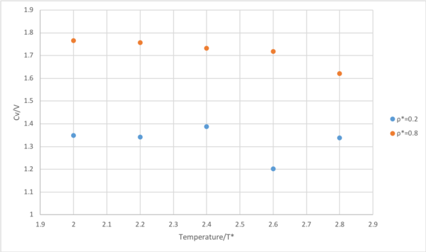
The plot indicates that the isochoric heat capacity decreases with increasing temperatures for ρ*=0.8. In a system of finite energy levels, there is a higher density of levels towards the energy maximum. At higher temperatures, electrons populate higher energy levels according to the Boltzmann distribution. Therefore, as energy level gap decreases, the thermal energy required to raise the internal energy by populating higher levels subsequently decreases. As $C_V=(\frac{\partial U}{\partial T}{)}_V$, the heat capacity decreases with increasing temperatures until all energy levels are equally occupied and it tends to infinity. Tends to infinity? As T -> inf, Cv -> 0. It becomes really hard to heat something up.

Whilst this trend is observed initially in the case of ρ*=0.2, the atoms go through a phase change, indicated by the rapid increase. At T*=2.4 all energy is converted to latent heat. After the phase change, the fluid can access further degrees of freedom such as vibration and rotation which would raise the heat capacity as they are an avenue for thermal energy. These extra degrees of freedom were unavailable at ρ*=0.8.

Furthermore, the heat capacity is consistently higher in the more dense system of ρ*=0.8 than ρ*=0.2 while obeying the same trend for temperature because the thermal energy must be distributed over a greater number of atomic energy levels per unit cell, requiring more energy.Tick

Radial Distribution Function

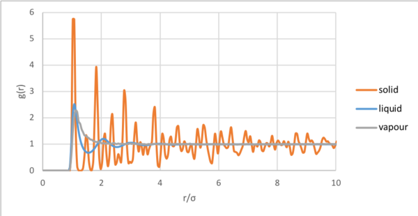
The radial distribution function (RDF) relates density to the radial distance from a reference atom . The RDF was determined for the solid, liquid and vapour phases. At short distances, $r<\sigma ,g(r)=0$ due interatomic repulsion, according to the Lennard-Jones potential. Eventually, the RDF for each of the three phases tended to 1, the bulk value. After reaching a maximum for the single coordination shell of a gas, $g(r)$ decays to 1. Although liquids are significantly more ordered than a gas, the radial distribution peaks for approximately the first three coordination shells and goes below 1 due to collisions before decaying. As liquids are dynamic, the peaks are broad and coordination shells are not correlated to the reference particle over long distances. The radial distribution function for the solid, displays regular maxima for the coordination spheres at $\sqrt{n}$ multiples of $\sigma$. The peak broadness results from atomic vibrations.

The radial distribution function.

The running integral of the radial distribution function

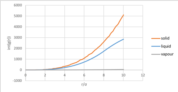The running integral, $\int (g(r)$ corresponds to the number of atoms at that radial distance by $n(r)=4\pi \rho \underset{0}{\overset{r^{\prime }}{\int }}g(r)r^{2}dr$ The coordination and number match the theoretical fcc model.

This region of the running integral plot shows the number of atoms in the first three coordination shells.

Data reported for lattice site coordination

Peak	Latice spacing	Intg(r)	Number of atoms	Coordination number
1	σ	12	12	12
2	√2 σ	18	6	12
3	√3 σ	42	24	12

fcc lattice illustrating atoms corresponding to peaks and radial diagram showing coordination shells for solid

Diffusion Coefficient: Mean Square Displacement

The mean squared displacement (MSD) gives the average deviation of a particle from a reference position. A logarithmic plot of MSD against step was generated to allow diagnosis of the ballistic and diffusion regions. After ln(step)=4, the particle motion changes from Brownian ballistic to Brownian diffusive . The three phases diverge as their degrees of freedom determine the extent to which the atoms can diffuse.

The total MSD for 1000 atoms against steps.

The total MSD for 1000000 atoms against steps.

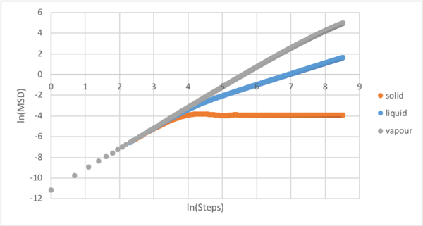The gradient in the diffusive region of the normal plot, the point at which lines diverge in the exponential plot, was determined and the diffusion coefficient calculated using the relationship $D=\frac{1}{6}\frac{\partial ⟨r^2\left(t\right)⟩}{\partial t}$.[See Tasks for compete plots] These values can be rationalised by theory. Atoms in a solid are restricted to one degree freedom, vibration, and so are not able to diffuse throughout the box. Liquid atoms are dynamic and experience limited translational motion allowing diffusion. Atoms in the vapour state, however, possess full translational freedom and so diffuse throughout the box. The difference between the 1000 and 100000 atom diffusion coefficients is caused by significantly greater averaging which reduces the effects of fluctuations on the simulation and considers a greater number of scenarios.

Data reported for diffusion coefficient determined from MSD

Number of Atoms	Solid	Liquid	Gas
1000	1.06x10-6	0.106	7.25
1000000	8.27x10-6	0.0873	3.01

Diffusion Coefficient: Velocity Auto-correlation Function

The diffusion coefficient was also determined from the velocity auto-correlation function (VACF). The VACF describes the extent to which an atoms' current velocity is correlated with its future velocity . It was evaluated analytically by considering the atoms as 1D harmonic oscillators and then compared to simulated VACF data.

$C\left(\tau \right)=⟨\mathbf{v}\left(t\right)\cdot \mathbf{v}(t+\tau )⟩$

$C\left(\tau \right)=\frac{\underset{-\mathrm{\infty }}{\overset{\mathrm{\infty }}{\int }}(-A\omega \sin (\omega t+\varphi )(-A\omega \sin (\omega (t+\tau )+\varphi ))\mathrm{d}t}{\underset{-\mathrm{\infty }}{\overset{\mathrm{\infty }}{\int }}(-A\omega \sin (\omega t+\varphi ){)}^2\mathrm{d}t}=\cos (\omega \tau )$

The VACF for the three states with the correlation function plotted. 1000 atoms.

The VACF for the three states with the correlation function plotted. 1000000 atoms

The analytic correlation predicted by the 1D harmonic oscillator maps similarly to the simulated VACF for solid and liquid initially but as they decay to zero it retains the sinusoidal pattern. This reflects the extent to which the atoms in the solid and liquid phases are able to oscillate around a fixed point like the 1D harmonic oscillator. Moreover, the simulated VACFs resemble the shape of the Lennard-Jones potential. The regularly structured solid vibrates around a fixed point but this reduced as the system tend to equilibrium. The translational motion of the liquid initially follows the same path as the 1D harmonic oscillator in the ballistic region but as diffusion begins to dominate its motion the VACF tends to 1. It also demonstrates the difference between the motion of liquid and solid: the solid undergoes vibrations and liquid undergoes diffusion. Introducing damping to the 1D harmonic oscillator would improve the fit. The minima in the VACF simulations are due to the change in direction of the atoms resulting from interatomic collisions.

The diffusion coefficient values estimated from the VACF by determining the area under the curve using the trapezium rule and applying the relationship $D=\frac{1}{3}\underset{0}{\overset{\mathrm{\infty }}{\int }}\mathrm{d}\tau ⟨\mathbf{v}\left(0\right)\cdot \mathbf{v}\left(\tau \right)⟩$

Data reported for diffusion coefficient determined from VACF

Number of Atoms	Solid	Liquid	Gas
1000	6.11x10-5	0.0979	8.45
1000000	4.55x10-5	0.0901	3.27

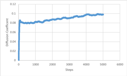
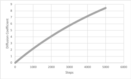
The results follow the same trends described for the calculation by MSD. The largest errors in the estimation of the diffusion coefficient from the area under the VACF is the trapezium rule and that the running integrals for vapour and solid do not converge to a limit [See Tasks for running integrals]. The trapezium rule estimates the area under a straight line connecting two points, ignoring the path taken between them. As this simulation produced a curve, an error results in measuring the area under it. Additionally, as the running integrals continued to increase for the liquid and vapour, the VACF has not converged to 0 and the diffusion coefficient is larger than that stated. This is less pronounced for 1000000 atoms, which suggests better averaging.

Conclusion

Imperial College's high performance computer was leveraged to perform molecular dynamic simulations in LAMMPS of atoms governed by Lennard-Jones interactions. It was found that number density was inversely proportional to temperature, although lower than that predicted by the ideal gas law. Heat capacity generally decreased with increasing temperature as higher atomic energy levels became occupied unless the atoms went through a phase change, which accessed further degrees of freedom. The impact of the dynamic capabilities of the atoms was also evident in the radial distribution function for solid, liquid and gas phases. The diffusion coefficients calculated for the three phases from the MSD and VACF data were in good agreement, which reflects the inherent link velocity and displacement measurements. Moreover, the MSD highlighted the transition from ballistic to diffusive motion and the VACF conveyed the rate of decay of velocity correlation over time, what was dependent on the atoms' dynamism.

Tasks

Theory

• Open the file HO.xls. In it, the velocity-Verlet algorithm is used to model the behaviour of a classical harmonic oscillator. Complete the three columns "ANALYTICAL", "ERROR", and "ENERGY": "ANALYTICAL" should contain the value of the classical solution for the position at time $t$, "ERROR" should contain the absolute difference between "ANALYTICAL" and the velocity-Verlet solution (i.e. ERROR should always be positive -- make sure you leave the half step rows blank!), and "ENERGY" should contain the total energy of the oscillator for the velocity-Verlet solution. Remember that the position of a classical harmonic oscillator is given by $x\left(t\right)=A\cos (\omega t+\varphi )$ (the values of $A$, $\omega$, and $\varphi$ are worked out for you in the sheet).
• For the default timestep value, 0.1, estimate the positions of the maxima in the ERROR column as a function of time. Make a plot showing these values as a function of time, and fit an appropriate function to the data.
• Experiment with different values of the timestep. What sort of a timestep do you need to use to ensure that the total energy does not change by more than 1% over the course of your "simulation"? Why do you think it is important to monitor the total energy of a physical system when modelling its behaviour numerically?

Absolute error between experimental and analytical values.

Percentage oscillation in energy for different timesteps.

• For a single Lennard-Jones interaction, $\varphi \left(r\right)=4ϵ(\frac{{\sigma }^{12}}{r^{12}}-\frac{{\sigma }^6}{r^6})$, find the separation, $r_0$, at which the potential energy is zero. What is the force at this separation? Find the equilibrium separation, $r_{eq}$, and work out the well depth ($\varphi \left(r_{eq}\right)$). Evaluate the integrals $\underset{2\sigma }{\overset{\mathrm{\infty }}{\int }}\varphi \left(r\right)\mathrm{d}r$, $\underset{2.5\sigma }{\overset{\mathrm{\infty }}{\int }}\varphi \left(r\right)\mathrm{d}r$, and $\underset{3\sigma }{\overset{\mathrm{\infty }}{\int }}\varphi \left(r\right)\mathrm{d}r$ when $\sigma =ϵ=1.0$.

$\varphi \left(r\right)=4ϵ(\frac{{\sigma }^{12}}{r_0^{12}}-\frac{{\sigma }^6}{r_0^6})=0$ when the potential energy is zero.

$\frac{{\sigma }^{12}}{r^{12}}=\frac{{\sigma }^6}{r^6}$

$r_0=\sigma$

To calculate the force at this separation $F=-\frac{d\varphi (r)}{dr}$

$F=-4ϵ(-\frac{12{\sigma }^{12}}{r_0^{13}}+\frac{6{\sigma }^6}{r_0^7})$

At $r=r_0=\sigma$, $F=-4ϵ(-\frac{12{\sigma }^{12}}{{\sigma }^{13}}+\frac{6{\sigma }^6}{{\sigma }^7})$

$F=\frac{24ϵ}{\sigma }$

Equilibrium occurs when the potential gradient is 0. $\frac{d\varphi (r)}{dr}=4ϵ(-\frac{12{\sigma }^{12}}{r_{eq}^{13}}+\frac{6{\sigma }^6}{r_{eq}^7})=0$

$\frac{12{\sigma }^{12}}{r_{eq}^{13}}=\frac{6{\sigma }^6}{r_{eq}^7}$

$r_{eq}=\sqrt[6]{2}\sigma$

The well depth at equilibrium is given by $\varphi \left(r_{eq}\right)=4ϵ(\frac{{\sigma }^{12}}{\sqrt[6]{2}{\sigma }^{12}}-\frac{{\sigma }^6}{\sqrt[6]{2}{\sigma }^6})$

$\varphi \left(r_{eq}\right)=4ϵ(\frac{1}{4}-\frac{1}{2})$

$\varphi \left(r_{eq}\right)=-ϵ$

Integrals. $\sigma =ϵ=1.0$

$\underset{2\sigma }{\overset{\mathrm{\infty }}{\int }}\varphi \left(r\right)\mathrm{d}r=\underset{2}{\overset{\mathrm{\infty }}{\int }}4(\frac{1}{r^{12}}-\frac{1}{r^6})\mathrm{d}r$

$=4{[-\frac{1}{11r^{11}}+\frac{1}{5r^5}]}_2^{\mathrm{\infty }}=-0.0248$

$\underset{2.5\sigma }{\overset{\mathrm{\infty }}{\int }}\varphi \left(r\right)\mathrm{d}r=\underset{2}{\int }.5^{\mathrm{\infty }}4(\frac{1}{r^{12}}-\frac{1}{r^6})\mathrm{d}r$

$=4{[-\frac{1}{11r^{11}}+\frac{1}{5r^5}]}_{2.5}^{\mathrm{\infty }}=-0.00818$

$\underset{3\sigma }{\overset{\mathrm{\infty }}{\int }}\varphi \left(r\right)\mathrm{d}r=\underset{3}{\overset{\mathrm{\infty }}{\int }}4(\frac{1}{r^{12}}-\frac{1}{r^6})\mathrm{d}r$

$=4{[-\frac{1}{11r^{11}}+\frac{1}{5r^5}]}_3^{\mathrm{\infty }}=-0.00329$

• Estimate the number of water molecules in 1ml of water under standard conditions. Estimate the volume of 10000 water molecules under standard conditions.

Water has a density of 1 g/mL and a molar mass of 18 g/mol. Thus there are 0.055 moles of water in 1 mL and 3.34x10²² molecules, found by multiplying the number of moles with Avagrado's constant (6.022x10²³). 1000 water molecules is equivalent 31.66x10^-22 moles, found by dividing by Avagrado's number. This is 2.99x10^-19 g and consequently 2.99x10^-19 mL.

• Consider an atom at position (0.5, 0.5, 0.5) in a cubic simulation box which runs from (0, 0, 0) to (1, 1, 1). In a single timestep, it moves along the vector (0.7, 0.6, 0.2). At what point does it end up, after the periodic boundary conditions have been applied?

The particle ends up at (0.2, 0.1, 0.7) after applying periodic boundary conditions to the position (1.2, 1.1, 0.7) achieved by vector addition.

• The Lennard-Jones parameters for argon are $$\begin{gathered} \sigma =0.34\mathrm{n}\mathrm{m},ϵ \\ / \\ {k}_B=120\mathrm{K} \end{gathered}$$. If the LJ cutoff is $r^{*}=3.2$, what is it in real units? What is the well depth in $$\begin{gathered} {\mathrm{k}\mathrm{J} \\ \mathrm{m}\mathrm{o}\mathrm{l}}^{-1} \end{gathered}$$? What is the reduced temperature $T^{*}=1.5$ in real units?

$r=r^{*}\sigma =3.2\times 0.32x10^{-9}=1.09nm$

$T=\frac{T^{*}{k}_b}{ϵ}=1.5\times 120=180K$

$ϵ=120k_b=120\times 1.38\times 10^{22}=1.66\times 10^{-21}=0.996kJmo{l}^{-1}$

Equilibration

• Why do you think giving atoms random starting coordinates causes problems in simulations? Hint: what happens if two atoms happen to be generated close together?

Random starting coordinates could generate atoms too close together, leading the atoms to unrealistically large interatomic repulsion and so velocities which would distort the simulation unless a very small timestep was used.

• Satisfy yourself that this lattice spacing corresponds to a number density of lattice points of 0.8. Consider instead a face-centred cubic lattice with a lattice point number density of 1.2. What is the side length of the cubic unit cell?

A face-centred cubic lattice contains has 4 atoms per unit cell.

${\rho }_N=\frac{N}{V}$

$1.2=\frac{4}{l^3}$

$l=1.49$

• TASK: Consider again the face-centred cubic lattice from the previous task. How many atoms would be created by the create_atoms command if you had defined that lattice instead?

1000 unit cells containing 4 atoms each would generate 4000 atoms.

• Using the LAMMPS manual, find the purpose of the following commands in the input script:

mass 1 1.0
pair_style lj/cut 3.0
pair_coeff * * 1.0 1.0

mass: atom type 1 with mass of 1.0

pair_style: Lennard-Jones potential between atom pairs ignoring coulombic interactions with the interaction cutoff at a separation of 3.0 A.

pair_coeff: for interactions between all atoms 1 to N, sigma and epsilon are set to 1.0.

• Given that we are specifying ${\mathbf{x}}_i\left(0\right)$ and ${\mathbf{v}}_i\left(0\right)$, which integration algorithm are we going to use?

Velocity-verlet

• Look at the lines below.

### SPECIFY TIMESTEP ###
variable timestep equal 0.001
variable n_steps equal floor(100/${timestep})
timestep ${timestep}

### RUN SIMULATION ###
run ${n_steps}
run 100000

The second line (starting "variable timestep...") tells LAMMPS that if it encounters the text ${timestep} on a subsequent line, it should replace it by the value given. In this case, the value ${timestep} is always replaced by 0.001. In light of this, what do you think the purpose of these lines is? Why not just write:

timestep 0.001
run 100000

Defining timestep as a variable allows the number of steps required to reach the set time for each timestep to be calculated by LAMMPS. This standardises the input file.

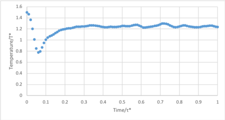
• Make plots of the energy, temperature, and pressure, against time for the 0.001 timestep experiment (attach a picture to your report). Does the simulation reach equilibrium? How long does this take? When you have done this, make a single plot which shows the energy versus time for all of the timesteps (again, attach a picture to your report). Choosing a timestep is a balancing act: the shorter the timestep, the more accurately the results of your simulation will reflect the physical reality; short timesteps, however, mean that the same number of simulation steps cover a shorter amount of actual time, and this is very unhelpful if the process you want to study requires observation over a long time. Of the five timesteps that you used, which is the largest to give acceptable results? Which one of the five is a particularly bad choice? Why?

A plot of total energy against time for timestep 0.001.

A plot of temperature against time for timestep 0.001.

A plot of pressure against time for timestep 0.001.

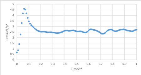The system reaches equilibrium at 0.4 τ*, indicated by the convergence of energy.

A comparison on the effect of timestep on energy convergence.

Timestep 0.015 fails to converge and increases constantly throughout the simulation. Additionally, the timesteps 0.01 and 0.075 are unsuitable as they converge to an incorrect energy value. Thus the only practicable timesteps are 0.0025 and 0.001. The largest acceptable timestep, 0.0025, is more computationally efficient than 0.001 without compromising significant accuracy.

Running Simulation over Specific Conditions

• Choose 5 temperatures (above the critical temperature $T^{*}=1.5$), and two pressures (you can get a good idea of what a reasonable pressure is in Lennard-Jones units by looking at the average pressure of your simulations from the last section). This gives ten phase points — five temperatures at each pressure. Create 10 copies of npt.in, and modify each to run a simulation at one of your chosen $(p,T)$ points. You should be able to use the results of the previous section to choose a timestep. Submit these ten jobs to the HPC portal. While you wait for them to finish, you should read the next section.

• We need to choose $\gamma$ so that the temperature is correct $T=\mathfrak{𝔗}$ if we multiply every velocity $\gamma$. We can write two equations:

$\frac{1}{2}\sum _i{m}_i{v}_i^2=\frac{3}{2}N{k}_{B}T$

$\frac{1}{2}\sum _i{m}_i{\left(\gamma v_i\right)}^2=\frac{3}{2}N{k}_B\mathfrak{𝔗}$

Solve these to determine $\gamma$.

$\frac{1}{2}\sum _i{m}_i{\left(\gamma v_i\right)}^2=\frac{1}{2}{\gamma }^2\sum _i{m}_i{\left(v_i\right)}^2$

Dividing $\frac{1}{2}{\gamma }^2\sum _i{m}_i{\left(v_i\right)}^2=\frac{3}{2}N{k}_B\mathfrak{𝔗}$ by $\frac{1}{2}\sum _i{m}_i{v}_i^2=\frac{3}{2}N{k}_{B}T$ gives

${\gamma }^2=\frac{\mathfrak{𝔗}}{T}$

$\gamma =\sqrt{\frac{\mathfrak{𝔗}}{T}}$

• Use the manual page to find out the importance of the three numbers 100 1000 100000. How often will values of the temperature, etc., be sampled for the average? How many measurements contribute to the average? Looking to the following line, how much time will you simulate?

fix_aves specifies Nevery, Nrepeat and Nfreq, in this case as the three numbers 100 1000 100000. An average is calculated every on timestep that is a multiple of Nfreq, using the directly preceding Nrepeat values that are multiples of Nevery and averaging over Nrepeat. If 1000000 timesteps are simulated in this experiment, 10 averages are calculated using the preceding 1000 numbers that are a multiple of 100 and dividing by 1000.

• When your simulations have finished, download the log files as before. At the end of the log file, LAMMPS will output the values and errors for the pressure, temperature, and density $\left(\frac{N}{V}\right)$. Use software of your choice to plot the density as a function of temperature for both of the pressures that you simulated. Your graph(s) should include error bars in both the x and y directions. You should also include a line corresponding to the density predicted by the ideal gas law at that pressure. Is your simulated density lower or higher? Justify this. Does the discrepancy increase or decrease with pressure?

The typeface is Myriad Pro.

The typeface is Myriad Pro.

The simulated number density for the fluid is higher than that predicted by the ideal gas law. The ideal gas model only considers perfectly elastic collisions between atoms and ignores electrostatic interactions. The simulated conditions includes pairwise Lennard-Jones potential that leads to repulsion between atoms at short distances. Hence the number of atoms per unit volume is less for the simulation than the ideal gas law. As the temperature increases, the discrepancy between the number densities decreases. At higher temperatures, the collision velocities are sufficient to overcome the intermolecular repulsive forces that dominate at lower temperatures as $v^2\alpha T$.

Calculating Heat Capacities using Statistical Physics

As in the last section, you need to run simulations at ten phase points. In this section, we will be in density-temperature $({\rho }^{*},T^{*})$ phase space, rather than pressure-temperature phase space. The two densities required at $0.2$ and $0.8$, and the temperature range is $2.0,2.2,2.4,2.6,2.8$. Plot $C_V/V$ as a function of temperature, where $V$ is the volume of the simulation cell, for both of your densities (on the same graph). Is the trend the one you would expect? Attach an example of one of your input scripts to your report.

Volume reduced isochoric heat capacity against temperature for ρ*=0.2 and 0.8.

The plot indicates that the isochoric heat capacity decreases with increasing temperatures for ρ*=0.8. In a system of finite energy levels, there is a higher density of levels towards the energy maximum. At higher temperatures, electrons populate higher energy levels according to the Boltzmann distribution. Therefore, as energy level gap decreases, the thermal energy required to raise the internal energy by populating higher levels subsequently decreases. As $C_V=(\frac{\partial U}{\partial T}{)}_V$, the heat capacity decreases with increasing temperatures until all energy levels are equally occupied and it tends to infinity.

Whilst this trend is observed initially in the case of ρ*=0.2, the atoms go through a phase change, indicated by the rapid increase. At T*=2.4 all energy is converted to latent heat. After the phase change, the fluid can access further degrees of freedom such as vibration and rotation which would raise the heat capacity as they are an avenue for thermal energy. These extra degrees of freedom were unavailable at ρ*=0.8.

Furthermore, the heat capacity is consistently higher in the more dense system of ρ*=0.8 than ρ*=0.2 while obeying the same trend for temperature because the thermal energy must be distributed over a greater number of atomic energy levels per unit cell, requiring more energy.

Heat Capacity Input ScriptFile:WdmnNvt 0.8 2.8.txt

Structural Properties and the Radial Distribution Function

• Perform simulations of the Lennard-Jones system in the three phases. When each is complete, download the trajectory and calculate $g(r)$ and $\int g(r)\mathrm{d}r$. Plot the RDFs for the three systems on the same axes, and attach a copy to your report. Discuss qualitatively the differences between the three RDFs, and what this tells you about the structure of the system in each phase. In the solid case, illustrate which lattice sites the first three peaks correspond to. What is the lattice spacing? What is the coordination number for each of the first three peaks?

The radial distribution function.

The running integral of the radial distribution function

The radial distribution function relates density to the radial distance from a reference atom. At short distances, $r<\sigma ,g(r)=0$ due interatomic repulsion, according to the Lennard-Jones potential. After reaching a maximum for the single coordination shell of a gas, $g(r)$ decays to 1. Although liquids are significantly more ordered than a gas, radial distribution peaks for approximately the first three coordination shells before tending to 1. As liquids are dynamic, the peaks are broad and coordination shells are not correlated to the reference particle over longer distances. The radial distribution function for the solid, displays regular maxima for the coordination spheres at $\sqrt{n}$ multiples of $\sigma$. The peak broadness results from atomic vibrations. The running integral, $\int (g(r)$ corresponds to the number of atoms at that radial distance by $n(r)=4\pi \rho \underset{0}{\overset{r^{\prime }}{\int }}g(r)r^{2}dr$

This region of the running integral plot shows the number of atoms in the first three coordination shells.

Data reported for lattice site coordination

Peak	Latice spacing	Intg(r)	Number of atoms	Coordination number
1	σ	12	12	12
2	√2 σ	18	6	12
3	√3 σ	42	24	12

fcc lattice illustrating atoms corresponding to peaks and radial diagram showing coordination shells for solid

Dynamical Properties and the Diffusion Coefficient

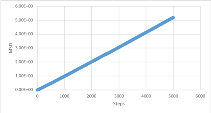
Make a plot for each of your simulations (solid, liquid, and gas), showing the mean squared displacement (the "total" MSD) as a function of timestep. Are these as you would expect? Estimate D in each case. Be careful with the units! Repeat this procedure for the MSD data that you were given from the one million atom simulations.

Mean Square Displacement against Time

Number of Atoms	Solid	Liquid	Vapour
1000
1000000

The gradient in the diffusive region (straight line) was determined and the diffusion coefficient calculated using the relationship $D=\frac{1}{6}\frac{\partial ⟨r^2\left(t\right)⟩}{\partial t}$. These values can be rationalised by theory. Atoms in a solid are restricted to one degree freedom, vibration, and so are not able to diffuse throughout the box. Liquid atoms are dynamic and experience limited translational motion allowing diffusion. Atoms in the vapour state, however, possess full translational freedom and so diffuse throughout the box. The difference between the 1000 and 100000 atom diffusion coefficients is caused by significantly greater averaging which reduces the effects of fluctuations on the simulation and considers a greater number of scenarios.

Data reported for diffusion coefficient determined from MSD

Number of Atoms	Solid	Liquid	Gas
1000	1.06x10-6	0.106	7.25
1000000	8.27x10-6	0.0873	3.01

In the theoretical section at the beginning, the equation for the evolution of the position of a 1D harmonic oscillator as a function of time was given. Using this, evaluate the normalised velocity autocorrelation function for a 1D harmonic oscillator (it is analytic!):

$C\left(\tau \right)=\frac{\underset{-\mathrm{\infty }}{\overset{\mathrm{\infty }}{\int }}v\left(t\right)v(t+\tau )\mathrm{d}t}{\underset{-\mathrm{\infty }}{\overset{\mathrm{\infty }}{\int }}{v}^2\left(t\right)\mathrm{d}t}$

Be sure to show your working in your writeup. On the same graph, with x range 0 to 500, plot $C\left(\tau \right)$ with $\omega =1/2\pi$ and the VACFs from your liquid and solid simulations. What do the minima in the VACFs for the liquid and solid system represent? Discuss the origin of the differences between the liquid and solid VACFs. The harmonic oscillator VACF is very different to the Lennard Jones solid and liquid. Why is this? Attach a copy of your plot to your writeup.

$=\frac{\underset{-\mathrm{\infty }}{\overset{\mathrm{\infty }}{\int }}(-A\omega \sin (\omega t+\varphi )(-A\omega \sin (\omega (t+\tau )+\varphi ))\mathrm{d}t}{\underset{-\mathrm{\infty }}{\overset{\mathrm{\infty }}{\int }}(-A\omega \sin (\omega t+\varphi ){)}^2\mathrm{d}t}$

$=\frac{\underset{-\mathrm{\infty }}{\overset{\mathrm{\infty }}{\int }}\frac{1}{2}(\cos (-\omega \tau )-cos(2\omega t+\omega \tau +2\varphi ))\mathrm{d}t}{\underset{-\mathrm{\infty }}{\overset{\mathrm{\infty }}{\int }}\frac{1}{2}(1-\cos (2\omega t+2\varphi ))\mathrm{d}t}$

$={\left[\frac{t\cos (-\omega \tau )-\sin (2\omega t+\omega \tau +2\varphi )\times \frac{1}{2\omega }}{t-\sin (2\omega t+2\varphi )\times \frac{1}{2\omega }}\right]}_{-\mathrm{\infty }}^{\mathrm{\infty }}$

$={\left[\frac{\cos (-\omega \tau )-\frac{1}{2\omega t}\sin (2\omega t+\omega \tau +2\varphi )}{1-\frac{1}{2\omega t}\sin (2\omega t+2\varphi )}\right]}_{-\mathrm{\infty }}^{\mathrm{\infty }}$

$=\frac{\cos (-\omega \tau )-0}{1-0}$

$=\cos (\omega \tau )$

The VACF for the three states with the correlation function plotted. 1000 atoms.

The VACF for the three states with the correlation function plotted. 1000000 atoms

The analytic correlation predicted by the 1D harmonic oscillator maps similarly to the simulated VACF for solid and liquid initially but as they decay to zero it retains the sinusoidal pattern. This reflects the extent to which the atoms in the solid and liquid phases are able to oscillate around a fixed point like the 1D harmonic oscillator. Moreover, the simulated VACFs resemble the shape of the Lennard-Jones potential. The regularly structured solid vibrates around a fixed point but this reduced as the system tend to equilibrium. The translational motion of the liquid initially follows the same path as the 1D harmonic oscillator in the ballistic region but as diffusion begins to dominate its motion the VACF tends to 1. It also demonstrates the difference between the motion of the liquid and solid: the solid undergoes vibrations and liquid undergoes diffusion. Introducing damping to the 1D harmonic oscillator would improve the fit. The minima in the VACF simulations are due to the change in direction of the atoms resulting from interatomic collisions.

Use the trapezium rule to approximate the integral under the velocity autocorrelation function for the solid, liquid, and gas, and use these values to estimate $D$ in each case. You should make a plot of the running integral in each case. Are they as you expect? Repeat this procedure for the VACF data that you were given from the one million atom simulations. What do you think is the largest source of error in your estimates of D from the VACF?

Diffusion Coefficient against Time for the Velocity Correlation Function

Number of Atoms	Solid	Liquid	Vapour
1000
1000000

Data reported for diffusion coefficient determined from VACF

Number of Atoms	Solid	Liquid	Gas
1000	6.11x10-5	0.0979	8.45
1000000	4.55x10-5	0.0901	3.27

The diffusion coefficient values estimated from the VACF by determining the area under the curve and applying the relationship $D=\frac{1}{3}\underset{0}{\overset{\mathrm{\infty }}{\int }}\mathrm{d}\tau ⟨\mathbf{v}\left(0\right)\cdot \mathbf{v}\left(\tau \right)⟩$ follow the same trends as the VACF. The results follow the same trends described for the calculation by MSD. The largest errors in the estimation of the diffusion coefficient from the area under the VACF is the trapezium rule and that the running integrals for vapour and solid do not converge to a limit. The trapezium rule estimates the area under a straight line connecting two points, ignoring the path taken between them. As this simulation produced a curve, an error results in measuring the area under it. Additionally, as the running integrals continued to increase for the liquid and vapour, the VACF has not converged to 0 and the diffusion coefficient is larger than that stated. This is less pronounced for 1000000 atoms, which suggests better averaging.

References

- ↑ M. Polanco, S. Kellas and K. Jackson, 65th Annu. Forum Proc. - AHS Int., 2009, 2, 1513–1524.
- ↑ S. V Garimella, T. Persoons, J. A. Weibel and V. Gektin, IEEE Trans. Components, Packag. Manuf. Technol., 2016, PP, 1191–1205.
- ↑ G. A. Cisneros, K. T. Wikfeldt, L. Ojamäe, J. Lu, Y. Xu, H. Torabifard, A. P. Bartók, G. Csányi, V. Molinero and F. Paesani, Chem. Rev., 2016, 116, 7501–7528.
- ↑ E. Cartlidge, New Sci.', 2010.
- ↑ M. C. Bellissent-Funel, A. Hassanali, M. Havenith, R. Henchman, P. Pohl, F. Sterpone, D. Van Der Spoel, Y. Xu and A. E. Garcia, Chem. Rev., 2016, 116, 7673–7697.
- ↑ P. Gallo, K. Amann-Winkel, C. A. Angell, M. A. Anisimov, F. Caupin, C. Chakravarty, E. Lascaris, T. Loerting, A. Z. Panagiotopoulos, J. Russo, J. A. Sellberg, H. E. Stanley, H. Tanaka, C. Vega, L. Xu and L. G. M. Pettersson, Chem. Rev., 2016, 116, 7463–7500.
- ↑ J.-P. Hansen and L. Verlet, Phys. Rev., 1969, 184, 151–161.
- ↑ M. I. Barker and T. Gaskell, J. Phys. C Solid State Phys., 2001, 5, 353–365.
- ↑ J. M. Seddon, Thermodynamics and statistical mechanics, Royal Society of Chemistry, Cambridge, 2001.
- ↑ R. Huang, I. Chavez, K. M. Taute, B. Lukić, S. Jeney, M. G. Raizen and E.-L. Florin, Nat. Phys., 2011, 7, 576–580.