Talk:Third year CMP compulsory experimenttg1412
Introduction
This experiment involved the investigation of a magnetic system and determining the effects of changing system size and the effect of changing the temperature, and determining the heat capacity and the Curie temperature.
Introducing the Ising Model
The Ising model, first proposed in the 1920s, is a simple model to explain the phase transition behaviour of systems with magnetic dipoles of variable spin states. This model is applied to a 2D lattice (in this experiment), which consists of multiple spins as elements which make up a 2D matrix. Each of these spins can have a value, +1 or -1 (spin pointing up or down respectively). When the spins are all alligned, that is to say, if they are all pointing in the same direction, the system is in its lowest energy state. It is an energetically favoured configuration. However, from a thermodynamic point of view, having all spins aligned leads to a decrease in entropy. Therefore, there is a constant compromise between energetic stability and entropic favourability. Each spin is assigned as si, and its neighbour spin is assigned sj. The energy comes from the interaction between the spins which are adjacent to each other when an external magnetic field is not applied. This interaction energy is defined as . is the interaction strength between the two spins, and is a constant for a specific system.
This energy is divided by two. This is to ensure that only one interaction is considered between each spin. si will interact with sj, and sj will equally interact with si. To remove this degenerate energy contribution, this factor of a half is included[3].
TASK: Show that the lowest possible energy for the Ising model is , where is the number of dimensions and is the total number of spins. What is the multiplicity of this state? Calculate its entropy.
Take a 3x3 lattice for example. Each edge of each unit which this lattice is made up from contributes to of energy to the system. On a square, every spin is interacting with its adjacent neighbours by four edges. So, the total energy contribution is . However, since 4 edges are shared, you are required to divide by two. This gives a total energy of . in this case, so the general energy is given by: . The entropy would be S = NKB ln2
NJ: Good, but you could do this "in general" by considering that in D dimensions there will be 2D neighbours for each cell. What is the multiplicity? (Alternatively, how do you get the entropy?)
TASK: Imagine that the system is in the lowest energy configuration. To move to a different state, one of the spins must spontaneously change direction ("flip"). What is the change in energy if this happens ()? How much entropy does the system gain by doing so?
In the lowest energy configuration, all spins will be aligned and in its ground state. So, you may use the equation , and the resulting energy given is . Flipping one spin will result in six anti-aligned interactions which will increase the energy of the system by . The resulting energy is thus , with an energy change of
The associated entropy change would be Sfinal state = NKB ln2000 / Sinitial state = NKB ln2 = NKB ln1000
NJ: It's actually +12J - you lose 6 "negative" interactions, but gain "positive" interactions.
TASK: Calculate the magnetisation of the 1D and 2D lattices in figure 1. What magnetisation would you expect to observe for an Ising lattice with at absolute zero?
 |
The magnetisation for the 1D and 2D lattices should be 1 and 1 respectively. This was calculated using the equation , where M is magnetisation. For a 3D lattice with N=1000, this should be in its ground state with all spins aligned at absolute zero, so the magnetisation should be (+ or -, depending on spin)1000.
Calculating the Energy and Magnetisation
The energy and magnetisation of a 2D lattice was examined. This 2D lattice was the used to model a chemical system. A random configuration for the lattice was created, with a special function that generated a random set of spins (random set of +1's and -1s's) for the lattice. The lattice itself was denoted by the variable self.lattice.
TASK: complete the functions energy() and magnetisation(), which should return the energy of the lattice and the total magnetisation, respectively. In the energy() function you may assume that at all times.
The code to calculate the energy is displayed below, and comments are made throughout to explain what the intention of specific important lines were.
def energy(self):
        <u>"Return the total energy of the current lattice configuration."</u>


        si_times_sj = [] '''# set up an empty list for the spins being multiplied, so a list of energies can be made'''
        for i in range(self.n_rows): '''#Use 'range' function to take into account all elements in the rows.'''
            for j in range(self.n_cols):
                '''#Top edge lattice values which are being multiplied by elements above (times by up)'''
                if i == 0:
                    si_times_sj.append(self.lattice[i,j]*self.lattice[self.n_rows-1,j]) '''#Here, I am saying that the last and first columns be multiplied and added to the list'''
                else: '''#For bulk of lattice elements not on edge'''
                    si_times_sj.append(self.lattice[i,j]*self.lattice[i-1,j])
                '''#Bottom edge lattice values which are being multiplied by elements above (times by bottom)'''
                if i == self.n_rows-1:
                     si_times_sj.append(self.lattice[i,j]*self.lattice[0,j])
                else: '''#For bulk of lattice elements'''
                    si_times_sj.append(self.lattice[i,j]*self.lattice[i+1,j])
                    '''#Left edge lattice values which are being multiplied by elements on left(times by left)'''
                if j == 0:
                    si_times_sj.append(self.lattice[i,j]*self.lattice[i,self.n_cols-1])
                else: '''#For bulk of lattice elements'''
                    si_times_sj.append(self.lattice[i,j]*self.lattice[i,j-1])
                    '''#Right edge lattice values which are being multiplied by elements on right(times by right)'''
                if j == self.n_cols-1:
                    si_times_sj.append(self.lattice[i,j]*self.lattice[i,0])
                else: '''#For bulk of lattice elements'''
                    si_times_sj.append(self.lattice[i,j]*self.lattice[i,j+1])


        Energy = -0.5*np.sum(si_times_sj) '''#The equation for energies.'''

        return Energy
This code returns the energy of the lattice.
The code below is written to calculate the total magnetisation for the lattice.
def magnetisation(self):
        <u>"Return the total magnetisation of the current lattice configuration."</u>

        M=0 #Magnetisation
        for i in range(self.n_rows):
            for j in range(self.n_cols):
                M += self.lattice[i,j] #Scanning through the entire lattice and increasing M by 1 each time
        return M
TASK: Run the ILcheck.py script from the IPython Qt console using the command
%run ILcheck.py
.
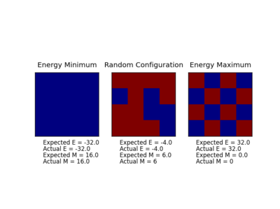 |
As you can see from the figure above, the codes work in agreement with the expected energy and magnetisation. Repeats were run of this code and each time the values produced were in harmony with the expected values.
Introducing the Monte Carlo simulation
Importance Sampling
Importance sampling is the technique of evaluating and calculating properties of a system which take up a specific distribution (of states, in our case). Since in a system, there will be many states existing, populating energy levels according to the Boltzmann exponential , not all of them will contribute greatly to the average energy and average magnetisation, and fortunately, these non contributing states make up quite a large sample that may be omitted in the final calculation. This will simplify and speed up the calculation significantly.
TASK: How many configurations are available to a system with 100 spins? To evaluate these expressions, we have to calculate the energy and magnetisation for each of these configurations, then perform the sum. Let's be very, very, generous, and say that we can analyse configurations per second with our computer. How long will it take to evaluate a single value of ?
A system of 100 spins will have 2100 configurations. That's 1.268 x 1030! For a computer which can analyse at a rate of 1 x 10⁹ configurations per second, to analyse 1.268 x 1030 will take 1.27 x 10²¹s to evaluate a single value of !
As you can see, even with a high processing power, it will take a significant amount of time to analyse the system containing 100 spins. The Monte Carlo algorithm first generates a configuration (or lattice) at random. The energy is then computed. One of the elements in the lattice will then have its spin "flipped". Again, this will be a completely random process. The energy of this new configuration is calculated, and if the change in energy is less than 0 (being a favourable energy change) then the new system of spins is accepted, because this was better than the original,and more stable. However, if the new energy is greater than 0, one of two things could happen. The probability of this spin flipping to its new state is given by the Boltzmann exponential. This new state will be accepted if a random number generated in the process falls below or equal to the probability of this spin flip. Otherwise, if this random number is greater than the probability of this spin flip, it will be rejected and the system will revert back to its original state, and the process will start again- generate a random lattice and proceed through the steps.
NJ: Nice explanation
TASK: Implement a single cycle of the above algorithm in the montecarlocycle(T) function. This function should return the energy of your lattice and the magnetisation at the end of the cycle. You may assume that the energy returned by your energy() function is in units of ! Complete the statistics() function. This should return the following quantities whenever it is called: , and the number of Monte Carlo steps that have elapsed.
The code written to execute a single Monte Carlo cycle is shown below, with comments made throughout to explain the intention of specific important lines.
def montecarlostep(self, T):
        <u># complete this function so that it performs a single Monte Carlo step</u>
        energy = self.energy()
        magnetisation = self.magnetisation()
        '''#the following two lines will select the coordinates of the random spin'''
        random_i = np.random.choice(range(0, self.n_rows))
        random_j = np.random.choice(range(0, self.n_cols))
        Energy_0 = self.energy() '''#Original energy'''
        self.lattice[random_i, random_j] = -1*self.lattice[random_i, random_j] '''#This will randomly select an element and flip its sign'''
        Energy_1 = self.energy() '''# New energy for flipped spin configuration'''
        dE = Energy_1 - Energy_0 '''#Change in energy'''

        if dE > 0: '''#Unfavourable energy change'''
            Probability = np.exp(-dE/T)
            random_number = np.random.random() '''#This line will choose a random number in the rang e[0,1)'''
            if random_number > Probability: '''#If unfavourable random number selection'''
                self.lattice[random_i, random_j] = -1*self.lattice[random_i, random_j] '''#Flipping spin back so original lattice can be returned'''

        self.n_cycles += 1 '''#Increase number of cycles run by 1'''
        self.E.append(self.energy())
        self.E2.append(self.energy() ** 2)
        self.M.append(self.magnetisation())
        self.M2.append(self.magnetisation() ** 2)

        return energy, magnetisation '''#Will return energy and magnetisation values. Since only one value can be returned, two variables A and B may be returned together by using "return A, B."'''
TASK: If , do you expect a spontaneous magnetisation (i.e. do you expect )?
If , spontaneous magnetisation would not be observed. It is only above the curie temperature were you will observe spontaneous magnetisation. At high temperatures, the entropy term dominates and spin flipping will be observed, increasing the entropy of the system with more anti aligned spins. At lower temperatures, the energy term dominates and aligned spins are favoured over anti aligned.
NJ: Increased preference for spin alignment leads to increased magnetisation, so below T_C we do expect to see it.
TASK:When the state of the simulation appears to stop changing (when you have reached an equilibrium state), use the controls to export the output to PNG and attach this to your report. You should also include the output from your statistics() function.
The figures above show the Monte Carlo simulation results. These show the energy per spin over a number of steps that have passed. they show that over an elapsed period of steps, the spin state tends towards -1 or +1. This alignment of spin states is confirmed by the top graphs (energy against steps) which shows the energy tending towards -2kb, ie, reducing to ground state.
The code below is the written for return of the values average energy, average energy squared, average magnetisation and average magnetisation squared.
def statistics(self):
        # complete this function so that it calculates the correct values for the averages of E, E*E (E2), M, M*M (M2), and returns them
        aveE = 0.0
        aveE2 = 0.0
        aveM = 0.0
        aveM2 = 0.0

        aveE = self.E/self.n_cycles #Average energy would be the energy divided by the number of cycles
        aveE2 = self.E/self.n_cycles
        aveM = self.M/self.n_cycles
        aveM2 = self.M2/self.n_cycles

        return aveE, aveE2, aveM, aveM2, self.n_cycles
NJ: Careful with the aveE2 line, it's returning <E>!
Accelerating the code
Python is a very good program to write code and perform analysis. However, its processing ability is very slow on its own. Luckily, there exists a very powerful package which provides support when using Python to sort large arrays and matrices of multiple dimensions. The previous energy and magnetisation functions have used multiple loops which individually scan over each spin. This current method takes up a lot of computational time. In the next exercise, this NumPy package has been used to accelerate the code. Hence it has been shown that using this NumPy module provides faster processing times of our 2D lattice of spins.
TASK: Look at the documentation for the NumPy sum function. You should be able to modify your magnetisation() function so that it uses this to evaluate M. The energy is a little trickier. Familiarise yourself with the NumPy roll and multiply functions, and use these to replace your energy double loop (you will need to call roll and multiply twice!).
The following code shows the change made to the previous energy code, and it is strikingly simpler in format.
def montecarlostep(self, T):
        def energy(self): '''#Changing energy code to find new, accelerated time'''
        energy = -1.0*np.sum(np.multiply(self.lattice, np.roll(self.lattice, 1, 0)))
        energy -= 1.0*np.sum(np.multiply(self.lattice, np.roll(self.lattice, 1, 1)))

        return energy
NJ: I guess the "def montecarlostep(self, T)"... line is just a copy/paste error? Where is the optimised magnetisation code?
Energy code
The np.roll function takes three arguments; the array (our lattice in this case), the number of places that the elements are chosen to shift by (a shift by one place is required, as the adjacent spin is the one being considered) and the axis of the returned list (0 in this case- an identical list is required as return). This NumPy function ensures the list is scanned through once, and when the terminal element on he right is reached, that the list is looped or "rolled" back to the beginning. This function generates a new list, only considers the elements to the right, and does no repeat over the same list. Once the row is complete and list generated, the next NumPy function np.multiply is executed. This function takes the lists and multiplies out the elements, generating another single list which has the product of each element in its array. The final NumPy function, np.sum, sequentially adds each element together, and produces a final value. This value is then multiplied by -1 (cf, original energy equation) and the final energy value is resulted.
Magnetisations code The same has been implemented for the magnetisations. The only subtle difference made here is the axis in the np.roll argument. Here, the axis has been set to 1. This setting will produce single elements (i.e., not an array). This is required, since then the np.multiply function will be effectively skipped and the function will simply sum each element generated. This is consistent with the original magnetisations equation.
The following figure confirms the attainment of correct energies and magnetisation %run ILanim.py
Averaged quantities: E = -8.45765930222 E*E = 84.1660593722 M = 0.0303739552029 M*M = 0.697116705639 n_cycles = -9700
The following figure provides a graphical illustration if these NumPy functions.
 |
NJ: Lovely explanation of roll!
TASK: Use the script ILtimetrial.py to record how long your current version of IsingLattice.py takes to perform 2000 Monte Carlo steps. This will vary, depending on what else the computer happens to be doing, so perform repeats and report the error in your average!
TASK: Use the script ILtimetrial.py to record how long your new version of IsingLattice.py takes to perform 2000 Monte Carlo steps. This will vary, depending on what else the computer happens to be doing, so perform repeats and report the error in your average!
The following table provides the computation times using the old and new energy codes, to run 2000 Monte Carlo steps, with standard error calculated. The standard error is smaller for the accelerated energy code.
| ||||||||||||||||||||||||||||||||||||||||||||
| ' | ' |
NJ: The standard error isn't associated with each of the measurements individually, it's a property of the set of measurements.
Using this new code is evidently quicker. It does not require the analysis of each individual spin. Also, it only takes into account one spin-spin interaction unlike the previous old energy code, which takes into account both interactions which then needs to be accounted for in the end. This new code with its implemented np.roll function means multiple for loops are not required to analyse all the spins in the lattice. Also, this new code calculated the energy and magnetisations in one line for each property unlike the previous codes which require multiple lines. For all these reasons and more, this accelerated code is much quicker.
The effect of temperature and system size
A system of N spins at temperature T eventually reaches an equilibrium state. In this part of the experiment, the behavior of different lattice sizes were examined at a certain temperature.
TASK: The script ILfinalframe.py runs for a given number of cycles at a given temperature, then plots a depiction of the final lattice state as well as graphs of the energy and magnetisation as a function of cycle number. This is much quicker than animating every frame! Experiment with different temperature and lattice sizes. How many cycles are typically needed for the system to go from its random starting position to the equilibrium state? Modify your statistics() and montecarlostep() functions so that the first N cycles of the simulation are ignored when calculating the averages. You should state in your report what period you chose to ignore, and include graphs from ILfinalframe.py to illustrate your motivation in choosing this figure.
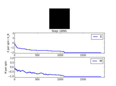
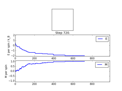
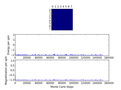
The following four plots show how long it took for each lattice size to reach equilibrium state at temperature set to 1.0
 |
 |
 |
 |
The square on the top of each of these plots show the final state of the system after a number of steps have passed. It shows the final state of the system reaching all aligned spins with the energy more or less fluctuating around -2. As you can see, for the larger 16x16 and 32x32 sizes, there is an initial "relaxation" period where the system starts off in a randomly selected state and takes a number of spins to reach minimum and fully aligned state. Larger lattice sizes take longer to reach equilibrium as there are more spins which need to be aligned. From the 32x32 plot, an approximate number of cycles of 50,000 was omitted and this number of cycles was removed for all lattices. The smaller lattice sizes seemed not to have this initial equilibration lag. The removal of this set of cycles was necessary; when the system is relaxing to the equilibrium state, these cycles will affect the average magnetisations and energies. To only take into account average energies and magnetisations, only average equilibrium fluctuations must be considered.
TASK: Use ILtemperaturerange.py to plot the average energy and magnetisation for each temperature, with error bars, for an lattice. Use your initution and results from the script ILfinalframe.py to estimate how many cycles each simulation should be. The temperature range 0.25 to 5.0 is sufficient. Use as many temperature points as you feel necessary to illustrate the trend, but do not use a temperature spacing larger than 0.5. T NumPy function savetxt() stores your array of output data on disk — you will need it later. Save the file as 8x8.dat so that you know which lattice size it came from.
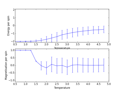
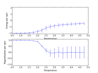
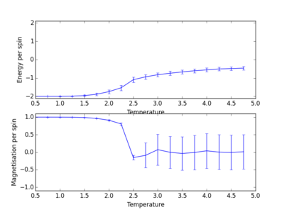
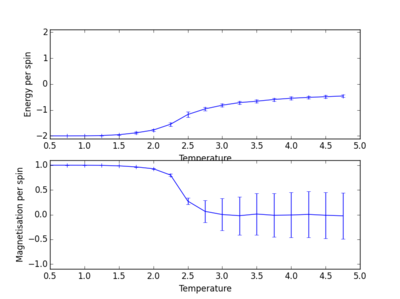
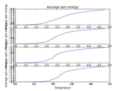
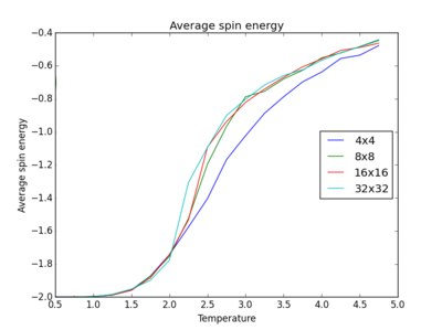
TASK: Repeat the final task of the previous section for the following lattice sizes: 2x2, 4x4, 8x8, 16x16, 32x32. Make sure that you name each datafile that your produce after the corresponding lattice size! Write a Python script to make a plot showing the energy per spin versus temperature for each of your lattice sizes. Hint: the NumPy loadtxt function is the reverse of the savetxt function, and can be used to read your previously saved files into the script. Repeat this for the magnetisation. As before, use the plot controls to save your a PNG image of your plot and attach this to the report. Below are the plots of average energies and magnetisations of each lattice size, with associated error bars.
The energy per spin was plotted versus temperature. As can be seen, the error in average energy per spin decreases with system size. However, the average magnetisation error stays roughly constant. As the temperature increases, the average energy per spin of the lattice system increases. A concurrent drop in magnetisation also occurs as the temperature is increased. This is suggestive of a phase transition. Spontaneous magnetisation occurs after a cutoff temperature. This temperature value is critical, and determines whether a material will show ferromagnetic behaviour. Looking at these plots, as the temperature of the system increases past this critical temperature, average magnetisation drops as average energy increases and spins become aligned in its ground state form[2].
 |
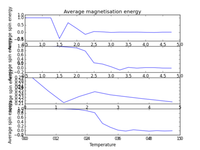 |
The plots above and below show the four different lattice sizes for comparison.
NJ: Attach the source for this one as well
 |
TASK: How big a lattice do you think is big enough to capture the long range fluctuations?
From the plots in the figures of average energies and error bars and overlayed plots above, it can be seen that larger lattice sizes deviate in error much much less than smaller lattice sizes. This shows that the larger 32x32 and 16x16 lattices head more towards an accurate answer to the average energy of the system. In general, bigger sample sizes are more representative of actual systems, and errors tend to be smaller. The smallest lattice size required to capture long range fluctuations should thus be given by the 8x8 lattice as this one, unlike the 4x4 lattice, better overlays with the larger lattice sizes at high temperature, as you can see from the figure above.
The following script was written to generate a plot of the lattice size against a set temperature to find energy and magnetisation per spin. Please note, that only the 4x4 lattice is shown in the code, the same process was executed for 8x8, 16x16 and 32x32. The script below shows the code executed to find the energy per spin variation with temperature. Even though this code was supplied, I have included it to show the minor change that had to be made with how the energies and magnetisations had to be ammended, due to the introduction of the global variable ignore.
NJ: Good
from IsingLattice import *
from matplotlib import pylab as pl
import numpy as np

n_rows = 4 #for a 4x4 lattice
n_cols = 4
il = IsingLattice(n_rows, n_cols)
il.lattice = np.ones((n_rows, n_cols))
spins = n_rows*n_cols
runtime = 150000 #Number of steps
times = range(runtime)
temps = np.arange(0.5, 5.0, 0.25) #starting temperature 0.5, final temperature 5.0 increasing in 0.25 increments
energies = [] #These variables had to be changed into empty lists due to global variable ''ignore''.
magnetisations = []
energysq = []
magnetisationsq = []
for t in temps:
    for i in times:
        if i % 100 == 0:
            print(t, i)
        energy, magnetisation = il.montecarlostep(t)
    aveE, aveE2, aveM, aveM2, n_cycles = il.statistics()
    energies.append(aveE)
    energysq.append(aveE2)
    magnetisations.append(aveM)
    magnetisationsq.append(aveM2)
    #reset the IL object for the next cycle
    #il = IsingLattice(n_rows,n_cols);

    il.E = [] #These variables had to be changed into empty lists.
    il.E2 =[]
    il.M = []
    il.M2 = []
    il.n_cycles = 0

fig = pl.figure()
enerax = fig.add_subplot(2,1,1)
enerax.set_ylabel("Energy per spin")
enerax.set_xlabel("Temperature")
enerax.set_ylim([-2.1, 2.1])
magax = fig.add_subplot(2,1,2)
magax.set_ylabel("Magnetisation per spin")
magax.set_xlabel("Temperature")
magax.set_ylim([-1.1, 1.1])
enerax.plot(temps, np.array(energies)/spins)
magax.plot(temps, np.array(magnetisations)/spins)
pl.show()

final_data = np.column_stack((temps, energies, energysq, magnetisations, magnetisationsq))
np.savetxt("4x4.dat", final_data)
The following script was written to plot the average energy and magnetisation against temperature. Although shown for the 4x4 lattice case, the same code was used for other lattice sizes.
from IsingLattice import *
from matplotlib import pylab as pl
import numpy as np

#4x4

four_by_four = np.loadtxt("4x4.dat")
temperature1 = four_by_four[:,0] #5 columns results in NumPy array, 1st column is temperature. This is used here.
average_E1 = four_by_four[:,1]/16 #5 columns results in NumPy array, 2nd column is average energy. This is used here.

fig=pl.figure()
pl.title("Average spin energy")

E_four_by_four = fig.add_subplot(4,1,1) #constructing subplots. 4 subplots, in a list.
E_four_by_four.set_xlabel("Temperature")
E_four_by_four.set_ylabel("Average spin energy")

E_four_by_four.plot(temperature1, average_E1)

pl.show()

#Magnetisation

#4x4

four_by_four = np.loadtxt("4x4.dat")
temperature1 = four_by_four[:,0]
average_E1 = four_by_four[:,3]/16 #5 columns results in NumPy array, 3rd column is average magnetisation. This is used here.

fig=pl.figure()
pl.title("Average magnetisation energy")

E_four_by_four_mag = fig.add_subplot(4,1,1)
E_four_by_four_mag.set_xlabel("Temperature")
E_four_by_four_mag.set_ylabel("Average spin energy")

E_four_by_four_mag.plot(temperature1, average_E1)

pl.show()
The statistics function, which returned average values, was modified to ignore the first selected N cycles. This is shown in the modified code below
ignore = 50000 #A global variable was created, called ignore. This variable was set to the number of cycles which were to be ignored for the plots to come
def statistics(self):
        # complete this function so that it calculates the correct values for the averages of E, E*E (E2), M, M*M (M2), and returns them
        aveE = 0.0
        aveE2 = 0.0
        aveM = 0.0
        aveM2 = 0.0

        temp = self.E[self.ignore:]
        aveE = np.average(temp)

        temp2 = self.E2[self.ignore:] #Ignore the first 10000.
        aveE2 = np.average(temp2)

        temp3 = self.M[self.ignore:]
        aveM = np.average(temp3)

        temp4 = self.M2[self.ignore:]
        aveM2 = np.average(temp4)

        return aveE, aveE2, aveM, aveM2, self.n_cycles - self.ignore
Takes longer for larger lattice sizes to reach equilibrium
NJ: Does that make sense?
Determining the heat capacity
In this part of the exercise, the heat capacity of the lattice sizes were plotted against temperature. The heat capacity is defined by the equation , where . As the temperature of the system, T, increases, the heat capacity of the system increases. More spins "flip" their spin states.
TASK: Write a Python script to make a plot showing the heat capacity versus temperature for each of your lattice sizes from the previous section. You may find that the data around the peak is very noisy — this is normal, and is a result of being in the critical region. As before, use the plot controls to save your a PNG image of your plot and attach this to the report.
NJ: It would be good to see all of these on the same axes (you would have to show the heat capacity per spin, of course)
 |
 |
 |
 |
These plots show the change in the peak region against an increasing temperature function as the system size gets progressively larger. The peak region becomes sharper towards a temperature value. The peaks become stronger as the system heads towards the vicinity of the Curie temperature.
NJ: What do you mean by this? The function becomes more strongly peaked as the lattice size increases, as formally becomes discontinuous for an infinite lattice.
The following script was written to plot heat capacity against temperature, and generate the graphs shown above. This code is demonstrated using the 32x32 lattice, but the same code was used for other lattice sizes also.
from IsingLattice import *
from matplotlib import pylab as pl
import numpy as np

thirtytwo_by_thirtytwo = np.loadtxt("32x32.dat") #Load the previously generated table of values.
temperature1 = thirtytwo_by_thirtytwo[:,0] #Using only the first column, which was temperature
average_E1 = thirtytwo_by_thirtytwo[:,1] #Using only the second column, which was average energy
average_sq_E1 = thirtytwo_by_thirtytwo[:,2] #Using only third column, which was average energy squared


variance = (average_sq_E1 - (average_E1 ** 2)) #Variance calculated
heat_capacity = variance /(temperature1 ** 2) #Heat capacity calculated

#print (heat_capacity) #This was just a check to ensure correct values


fig=pl.figure() #Plotting figure
pl.title("Heat Capacity v Temperature") #Title of figure

H_thirtytwo_by_thirtytwo = fig.add_subplot(4,1,1) #Want four sub plots
H_thirtytwo_by_thirtytwo.set_xlabel("Temperature") #X axis
H_thirtytwo_by_thirtytwo.set_ylabel("Heat Capacity") #Y axis

H_thirtytwo_by_thirtytwo.plot(temperature1, heat_capacity) #Plot


pl.show() #Show plot
Locating the Curie Temperature
The C++ program is much faster at processing larger simulations that take a longer time to process. This is due to its compiled nature. These data have been compared with those generated using Python in this section of the report.
TASK: A C++ program has been used to run some much longer simulations than would be possible on the college computers in Python. Each file contains six columns: (the final five quantities are per spin), and you can read them with the NumPy loadtxt function as before. For each lattice size, plot the C++ data against your data. For one lattice size, save a PNG of this comparison and add it to your report.
The figure below is a comparison of the heat capacity v temperature graph plotted using Python and compared against C++. As you can see, C++ is able to gather more data points, and have much smaller incremental increase in temperature, and the peak of the plot is sharper and more precise.
NJ: Good. It might have been clearer if you had used points to represent the python data, rather than a line.
 |
Below, I have only given the code written to construct the 32x32 lattice. The same was carried out for all other lattice sizes too.
from IsingLattice import *
from matplotlib import pylab as pl
import numpy as np

#Python graphs for 32x32 lattice

thirtytwo_by_thirtytwo = np.loadtxt("32x32.dat") #Load Python data
temperature1 = thirtytwo_by_thirtytwo[:,0] #Only include temperature in this variable
average_E1 = thirtytwo_by_thirtytwo[:,1] #Only include average energy in this variable
average_sq_E1 = thirtytwo_by_thirtytwo[:,2] #Only include average energy squared in this variable


variance = (average_sq_E1 - (average_E1 ** 2))/1024 #Variance is divided by the total number of spins in lattice
heat_capacity = variance /(temperature1 ** 2)

#print (heat_capacity) #Just a check for values, but commented out


fig=pl.figure() #Plotting graphs
pl.title("Heat Capacity v Temperature")

H_thirtytwo_by_thirtytwo = fig.add_subplot(1,1,1)
H_thirtytwo_by_thirtytwo.set_xlabel("Temperature")
H_thirtytwo_by_thirtytwo.set_ylabel("Heat Capacity")

H_thirtytwo_by_thirtytwo.plot(temperature1, heat_capacity)

#pl.show()

#C++ graphs lattice

thirtytwo_by_thirtytwo_C = np.loadtxt("C32x32.dat") #Load C++ data

temperature_C = thirtytwo_by_thirtytwo_C[:,0] #Only include temperature in this variable
heat_capacity_C = thirtytwo_by_thirtytwo_C[:,5] #Only include heat capacity in this variable

'''
H_thirtytwo_by_thirtytwo_C = fig.add_subplot(1,1,1) #These are unneeded so have been commented out but not deleted (I have separation anxiety)
H_thirtytwo_by_thirtytwo_C.set_xlabel("Temperature")
H_thirtytwo_by_thirtytwo_C.set_ylabel("Heat Capacity")'''

H_thirtytwo_by_thirtytwo.plot(temperature1, heat_capacity, label = "32x32")
H_thirtytwo_by_thirtytwo.plot(temperature_C, heat_capacity_C, label = "32x32")

pl.legend(loc=5)
pl.show()
NJ: Yes, it's always good to keep code around until you're **really** sure you don't need it...
'Fitting the polynomial and locating the Curie temperature'
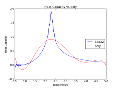
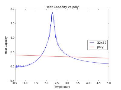
TASK: write a script to read the data from a particular file, and plot C vs T, as well as a fitted polynomial. Try changing the degree of the polynomial to improve the fit — in general, it might be difficult to get a good fit! Attach a PNG of an example fit to your report.
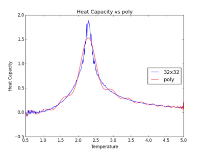
The figures below show the degree to which the polynomial implemented fit the heat capacity v temperature curves.
As you increase the order of the polynomial, the fit does improve, however, it is not perfect. There are still large deviations between the peak of the plot and the fitted polynomial. The order of the polynomial fitting can go on indefinitely but once the order has reached the system size, one cannot fit the polynomial to any higher degree. This imposes a practical problem when manually trying to fit a polynomial to such a graph.
Below is the script written to generate the fitted polynomial. The 200th order polynomial has been demonstrated here.
from IsingLattice import *
from matplotlib import pylab as pl
import numpy as np

data = np.loadtxt("C32x32.dat") #assume data is now a 2D array containing two columns, T and C, from C++ data files
T = data[:,0] #get the first column
C = data[:,5] # get the second column

#first we fit the polynomial to the data
fit = np.polyfit(T, C, 200) # fit a 200th order polynomial

#now we generate interpolated values of the fitted polynomial over the range of our function
T_min = np.min(T)
T_max = np.max(T)
T_range = np.linspace(T_min, T_max, 1000) #generate 1000 evenly spaced points between T_min and T_max
fitted_C_values = np.polyval(fit, T_range) # use the fit object to generate the corresponding values of C


fig=pl.figure()
pl.title("Heat Capacity vs poly")


H_poly = fig.add_subplot(1,1,1)
H_poly.set_xlabel("Temperature")
H_poly.set_ylabel("Heat Capacity")

H_poly.plot(T, C, label = "32x32")

H_poly.plot(T_range, fitted_C_values, label = "poly")


pl.legend(loc=5)
pl.show()
'Fitting the polynomial over required range, on C++ data'
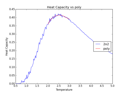
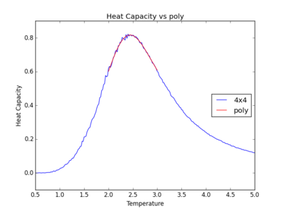
TASK: Modify your script from the previous section. You should still plot the whole temperature range, but fit the polynomial only to the peak of the heat capacity! You should find it easier to get a good fit when restricted to this region.
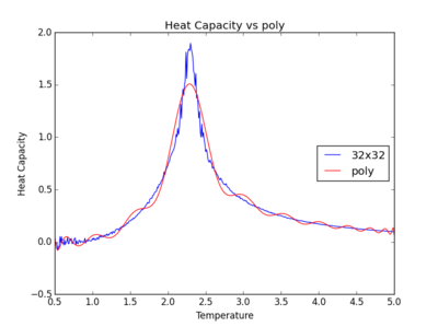
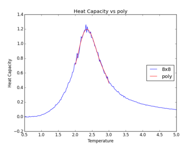
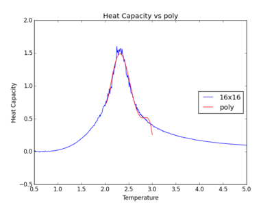
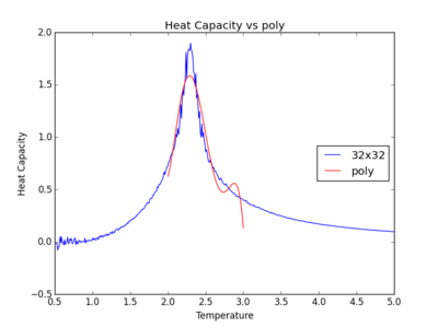
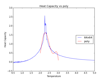
Below are the plots with polynomials fitted only around the required peak region.
NJ: For the larger lattices, the peak doesn't quite fit. It looks like the minima are slightly lower in temperature than the truer minima - perhaps changing the temperature range would help.
It can be observed that the polynomials fit the peaks better when only subjected to this temperature range spanning the peak region. However, as the lattice size gets larger, the peak becomes sharper. For an infinite lattice, the peak actually diverges at T = TC, so the polynomial for the larger 32x32 and 64x64 lattices do not fit as well.
Below is the code written to execute the graphs and specific polynomial fitting.
from IsingLattice import *
from matplotlib import pylab as pl
import numpy as np

data = np.loadtxt("C32x32.dat") #assume data is now a 2D array containing two columns, T and C
T = data[:,0] #get the first column
C = data[:,5] # get the second column

T_min = 2 #Minimum temperature to start fitted polynomial from
T_max = 3 #Maximum temperature to end fitted polynomial on.

selection = np.logical_and(T > T_min, T < T_max) #choose only those rows where both conditions are true
peak_T_values = T[selection]
peak_C_values = C[selection]

fit = np.polyfit(peak_T_values, peak_C_values, 5)
T_range = np.linspace(T_min, T_max, 1000)
fitted_C_values = np.polyval(fit, T_range)

fig=pl.figure()
pl.title("Heat Capacity vs poly")


H_poly_fit = fig.add_subplot(1,1,1)
H_poly_fit.set_xlabel("Temperature")
H_poly_fit.set_ylabel("Heat Capacity")

H_poly_fit.plot(T, C, label = "32x32")

H_poly_fit.plot(T_range , fitted_C_values, label = "poly")

pl.legend(loc=5)
pl.show()
Finding the Curie temperature
The following table shows the Curie temperature located for each lattice size. The maximum of the polynomial plot was found. These values, and value for heat capacity are shown below.
As the lattice size increases, the value of the Curie temperature becomes smaller and closer to 2.28. No apparent pattern can be seen for the heat capacity varying with temperature because as the system size becomes larger, the peak becomes sharper but more noisy, resulting in erratic sharp peaks. Also, since the polynomial fit is not as good for larger lattice sizes, an incorrect value of heat capacity will be reported. This inconsistency is shown by the fluctuations of heart capacities calculated. The peak height fluctuates a lot as system size gets larger.
The code written to plot the Curie temperature is shown below.
from IsingLattice import *
from matplotlib import pylab as pl
import numpy as np


#64x64 C++
data = np.loadtxt("C64x64.dat") #assume data is a 2D array containing two columns, T and C, from C++ data
T = data[:,0] #get the first column containing temperature
C = data[:,5] # get the 6th column containing heat capacity for 64x64

T_min = 2 #Set min and max temperatures
T_max = 2.5

selection = np.logical_and(T > T_min, T < T_max) #choose only those rows where both conditions are true
peak_T_values_64x64 = T[selection]
peak_C_values_64x64 = C[selection]

fit = np.polyfit(peak_T_values_64x64, peak_C_values_64x64, 200) #200th order polynomial fitted.
peak_T = np.linspace(T_min, T_max, 1000)
fitted_C_values_64x64 = np.polyval(fit, peak_T)

fig=pl.figure()
pl.title("Heat Capacity vs poly")


H_poly_fit_64x64 = fig.add_subplot(1,1,1)
H_poly_fit_64x64.set_xlabel("Temperature")
H_poly_fit_64x64.set_ylabel("Heat Capacity")

H_poly_fit_64x64.plot(T, C, label = "64x64")

H_poly_fit_64x64.plot(peak_T , fitted_C_values_64x64, label = "poly", color = "r")


pl.legend(loc=5)
pl.show()


Cmax = np.max(fitted_C_values_64x64)
Tmax = peak_T[fitted_C_values_64x64 == Cmax] #Print maximum temperature and heat capacity
print (Tmax, Cmax)
TASK: find the temperature at which the maximum in C occurs for each datafile that you were given. Make a text file containing two colums: the lattice side length (2,4,8, etc.), and the temperature at which C is a maximum. This is your estimate of for that side length. Make a plot that uses the scaling relation given above to determine . Discuss briefly what you think the major sources of error are in your estimate.
The equation which shows how heat capacity maximum is scaled as a function of temperature is given by the equation . is the Curie temperature, is the LxL lattice size used and is the Curie temperature of an infinite lattice.
 |
The Curie temperature of each lattice was plotted against 1 over lattice length. A line of best fit was then plotted, with the y intercept being equal to the Curie temperature of an infinite lattice. The Curie temperature from this plot was found to be 2.286 to 3dp.
NJ: Again, I'd represent the T_C values by points, and the fitted function with a line.
The code written to plot this graph is shown below.
from IsingLattice import *
from matplotlib import pylab as pl
import numpy as np

T_C = [2.519879825,2.44914915,2.33303303,2.31931932,2.2987988,2.28528529] #List of Curie temperatures from each lattice size.
L = [0.5,0.25,0.125,0.0625,0.03125,0.015625] # The value of the reciprocal of lattice side length. A was chosen to be equal to 1 for clarity
fit = np.polyfit(L, T_C, 1) #Fit polynomial plot to first order to get y intercept value.
L_range = np.linspace(0, 0.5, 1000)
fitted_C_values = np.polyval(fit, L_range)
fig=pl.figure()
pl.title("Curie Temperature")
Curie = fig.add_subplot(1,1,1)
Curie.set_xlabel("Lattice length")
Curie.set_ylabel("Tc")
Curie.plot(L, T_C, label = "Tc from plots")
Curie.plot(L_range, fitted_C_values, label = str(fit[1]) + " = Curie infinite")
pl.legend(loc=5)
pl.show()

print (fit[1])
The literature value of the Curie temperature was found to be 2.269[1]
TASK: Discuss briefly what you think the major sources of error are in your estimate.
The computers used to run these calculations are not capable of running a large number of steps, using Python (an interpreted language) unlike C++ which is a compiled language, and able to store bits of memory in its cache, allowing for faster processing. Since not being able to run a large number of steps using Python, this poses an obvious source of error in the final value of heat capacity obtained as the polynomial fit will be different.
NJ: But the final data you fitted was from the C++ simulations!
The a polynomial is being fitted to a plot which we assume to be polynomial. A polynomial was fitted to nth order until it seemed like it was a good enough fit, all by eye. This is a possible source of error, as we do not know for sure whether these heat capacity versus temperature plots follow a polynomial order. Following from this, the polynomial fit becomes less and less good for larger lattice sizes, as has been explained already, due to its diverging property as temperature tends towards the Curie temperature.
NJ: What about looking at larger lattices, or ignoring the small ones?
References
[1] J. Kotze, arXiv, 2008, p22
[2] D. K. Khudier, N. I. Favas, Int. Lett. of Chem. Phys. and Astr, 2013, 10(2), p201-212
[3] https://wiki.ch.ic.ac.uk/wiki/index.php?title=Third_year_CMP_compulsory_experiment as accessed on 15/03/2015 at 22:52

