Talk:Third Year Liquid Simulations KKL115

Overall: not bad - things to improve. Slow down and think through explanations a little more. You are really good at explaining ideas just need to put pen to paper! Also read through and check for grammar. Mark: 64/100

Abstract

Not a bad attempt at an abstract - but you need to state your purpose Simulations of Lennard-Jones liquids, solids and vapours were run on the LAMMPS application on the HPC supercomputer in order to determine the variation of number density and heat capacity with temperature, calculate the radial distribution function to determine the coordination of the structures and determine the diffusion coefficient using the mean squared distribution and the velocity autocorrelation function. for what purpose? It was found that number density increased with pressure but had an inverse relationship to temperature. (called equation of state) Heat capacity decreased as temperature increased but was higher for greater densities for a fixed volume. The radial distribution function affirmed that solids had the most ordered structure with gases being the most disordered as the most diffuse and the solid lattice spacing was found to be 1.175. Liquids fell in between the two but maintain a short range coordination sphere. The diffusion coefficient for both the mean squared distribution (MSD) and velocity autocorrelation function (VACF) were of a similar order of magnitude with the diffusion coefficients (units?): Gas = 1.16 (MSD), 7.70 (VACF); Liquid = 0.504 (MSD), 0.098 (VACF); Solid = 0.0005 (MSD), 0.0001 (VACF). Both the liquid and solid were correlated although the oscillatory behaviour decayed quicker for the liquid than the solid. It was surmised that the VACF values were less accurate as the running integrals for gas and liquid did not converge and because the trapezium rule approximation could not be fitted exactly to the curves so would have given a smaller value than determined.

Introduction

An interesting overview of liquids and specifically water. We need to ensure that the introduction ties in with everything and creates the dialogue. What are we doing in this experiment? We're calculating the phase properties. Thus, this is something we should concentrate on in our intro. Why are phase properties interesting but also relevant for research. With liquids being one of the four states of matter (the others being gas, solid and plasma), it is surprising given its prevalence on Earth that it should be relatively rare outside out it(? gram), with gas forming the majority of known matter. Water is ubiquitous to humans and yet it is gram liquid of contradictions and anomalies. Many of its unusual properties are due to the intermolecular hydrogen bonding network which are gram responsible for the density of ice being less than liquid water and the high surface tension responsible for the droplets of water seen as rain almost everyday.

The electronegativity of the oxygen atom polarises the molecule, leaving the hydrogen atom with a partial positive charge and allows the hydrogen bonding network to be formed via interactions with lone pairs on other nearby oxygen atoms. This network in turn fluctuates due to the dynamic nature of liquids moving and the hydrogen bonds will break and reform constantly. However, upon formation of ice the hydrogen bonds are locked in a rigid network and the molecules are held in a lattice further apart than they would have been in liquid form, due to the length of hydrogen bond at 1.97 Å compared to the 0.96 Å O-H bond length in water reducing its density to less than 1g per ml.

Hydrogen bonding is responsible for many unusual properties of water. The diffusion of protons and hydroxide ions are unusually fast in aqueous solutions due to their ability to be transported via the Grotthus Mechanism. The ions can transfer from one water molecule to the next via the rearrangement of the hydrogen bonds allowing them to have an unusually high mobility. Additionally, the high specific heat capacity of water is related to the hydrogen bonds that are required to be broken for the liquid to increase in temperature and they are the reason for the formation of water droplets. Liquids form spherical shapes for the smallest surface area to volume ratio and for water, the surface tension is high due to the relative strength of hydrogen bonds compared to other intermolecular attractive forces. The high surface tension allows the surface area of the droplet to be minimised so individual molecules within the liquid can interact with the maximum number of surrounding molecules. Tick, good

However, pressurised water between 100 °C - 374 °C undergoes a phenomenon known as superheating. Under these conditions, hydrogen bonds break leading to a decrease in the anomalous behaviour of water; the polarity, surface tension and viscosity decrease.

Furthermore, a contrasting phenomena known as super cooling can lead to the formation of a different solid phase, bypassing the crystalline ice structure completely. Pure water can be supercooled as without the presence of a nucleus to form a crystal structure, an amorphous solid known as glassy water will form. Tick

Methods

Be sure to highlight your units! All experimental graphs have been plotted in Python and all simulations run through the LAMMPS application via the HPC portal as Lennard-Jones systems.

The simulations for the Equations of State were run under an npt ensemble. The pressures chosen were 2.5 and 3.5, reasonable values in Lennard-Jones units as they were in the same order of magnitude to the equilibration step of the experiment. The temperatures: 2.0, 5.0, 7.5, 9.0. 10.0. These simulations were run with a timestep of 0.001, as chosen during the equilibration to ensure that the simulations would converge in a suitable timescale. A simple cubic lattice structure was chosen as fluids were being simulated, above the critical T=1.5 and a graph plotted of the number density against temperature. I don't understand?

The heat capacity was found using the following input script for densities of 0.2 and 0.8 and a range of temperatures of 2.0, 2.2, 2.4, 2.6, 2.8:

The input file for number density=0.2 and T=2.0 to calculate heat capacity

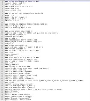
The input script defines the variable density and the crystal is melted under the thermodynamic conditions nve, fixing the number of particles, volume and energy. However, given that heat capacity is the change in magnitude of energy relative to thermal energy, the system was placed under the nvt ensemble during the measurement of the system state. This allowed the energy to vary and the temperature to remain constant.Tick For similar reasons to the equation of state procedure, a timestep of 0.001 and simple cubic lattice were used. The variance in energy and average temperature were calculated by the simulation and with the values given, the equation below was used to calculate heat capacity:

$C_V=\frac{\partial E}{\partial T}=\frac{\mathrm{V}\mathrm{a}\mathrm{r}\left[E\right]}{k_B{T}^2}=N^2\frac{⟨E^2⟩-{⟨E⟩}^2}{k_B{T}^2}$

$\mathrm{V}\mathrm{a}\mathrm{r}\left[E\right]$ is the variance in $E$, $N$ is the number of atoms. 'The $N^2$ is required because LAMMPS divides all energy output by the number of particles'. Then $\frac{C_v}{V}$ was plotted against temperature to observe how heat capacity varied.

The radial distribution functions (RDF) were calculated using the VMD programme from the University of Illinois. (cite) The trajectories were downloaded from the HPC Portal to calculated the RDF and the integral for the RDF plot, then analysed in Python to give the structures and coordinations of the solid, liquid and gas.

Diffusion coefficients were calculated using $D=\frac{1}{6}\frac{\partial ⟨r^2\left(t\right)⟩}{\partial t}$ with the gradients of the mean squared displacement graphs and using the velocity autocorrelation function whereby the calculations were peformed using $D=\frac{1}{3}\underset{0}{\overset{\mathrm{\infty }}{\int }}\mathrm{d}\tau ⟨\mathbf{v}\left(0\right)\cdot \mathbf{v}\left(\tau \right)⟩$. Instead of using the gradient, the trapezium rule was applied to approximate the VACF integral by taking the area under the plot to find $D$.Tick

Results and Discussion

Equations of State

Pressure=2.5

Pressure=3.5

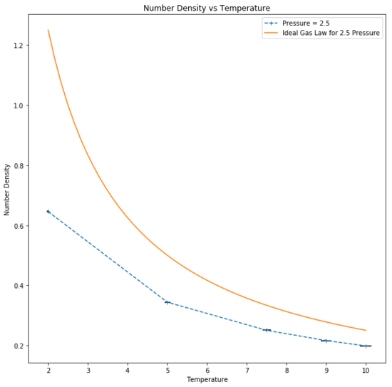
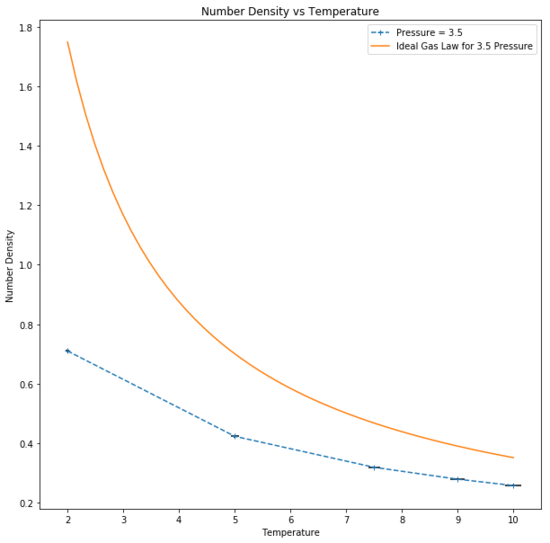
Number density, defined as $\frac{N}{V}$ was found to have an inverse relationship with temperature, as expected from the reduced unit ideal gas law: $\frac{N}{V}=\frac{p}{T}$

An ideal gas is assumed to have zero interactions with other particles, point particles and the Lennard-Jones parameter "a" and "b" set to zero, hence indicating that there would be no interactions between particles. The simulated number density deviates from ideality as the thermodynamic system for the simulation was run under the assumption that Lennard-Jones interactions between atom pairs exist, leading to attractive and repulsive forces between particles. Repulsion occurs at short distances between the particles which occurs upon interaction of the particles. Thus, the particles are on average further apart and there are fewer in a given volume, leading to a lower density.Good

At higher temperatures, the particles have greater kinetic energy and are able to move further away to reduce repulsion as much as possible. Therefore on average the particles are further apart than they would be at a lower temperature and lead to increased ideality as particle interaction is reduced. At low temperatures, the opposite is true and the increased interaction causes a large deviation from ideal behaviour as density increases. Tick

Additionally, at higher pressures it can be seen that the number density in a given area is greater than at a lower pressure and so interaction increases, tending further from ideality. This is due to the reduced volume to which the particles are confined and the particles undergo a larger number of collisions. It follows that the increased interaction leads to a larger deviation from ideal behaviour as a result of the increased repulsion.Good

Heat Capacity

Be sure to define your ensemble... These are rather dramatic so explain why :^)

Plot for heat capacity/volume against temperature for number density=0.2 ran as a simple cubic lattice

Plot for heat capacity/volume against temperature for number density=0.8 ran as a simple cubic lattice

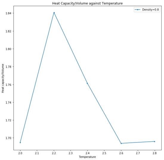
Heat capacity is defined as the variance in the total energy of the system, relative to the thermal energy put in and therefore indicates that a system with a large heat capacity would display only a small change in temperature as given by: Be careful with your definitions... heat capacity varies with variance in total energy etc but is fundamentally a measure of how easy it is to heat something up

$C_V=\frac{\partial E}{\partial T}=\frac{\mathrm{V}\mathrm{a}\mathrm{r}\left[E\right]}{k_B{T}^2}=N^2\frac{⟨E^2⟩-{⟨E⟩}^2}{k_B{T}^2}$

The trend observed of the inverse relationship between heat capacity and temperature was expected as dictated by the Boltzmann Distribution:

$\frac{N_i}{N}=\frac{e^{-{\epsilon }_i/kT}}{\sum _{j=1}^M{e}^{-{\epsilon }_j/kT}}$

In general, the population of higher energy vibrational modes are less probable than the population of lower energy states. Tick However, when temperature increases, the system obtains increased degrees of freedom and the thermal energy put into the system increases. Subsequently, higher energy states can be occupied more easily as the internal energy of a system increases when temperature is raised. Assuming that the particles in the system behave as anharmonic oscillators ooft but I'm not sure I follow, the energy levels will converge and the higher the energy, the closer they are. This means that when the higher energy states are occupied, the heat capacity decreases as the fluctuation in the total energy of the system will be small relative to the change in thermal energy and so heat capacity is observed to have an inverse relationship with temperature.

Additionally, the observed trend of an increased heat capacity with density is a consequence of the fixed volume system. An increased density therefore means that there are a greater number of particles in a given volume for a given quantity of thermal energy provided at a set temperature.An increased density doesn't really have anything to do with thermal energy or temperature... Over a larger number of particles, the average internal energy of the system is therefore lower and the higher energy states are less likely to be populated. Thus any excitation to a higher energy level would require more thermal energy to be put into the system and the variance of the total system energy would be large relative to the thermal energy put in (increased heat capacity).

There are two anomalies in the trend that are unexpected at $T^{*}=2.2,2.6$ for both densities. Given that the thermodynamic parameters ensured that the crystal was melted before the other thermodynamic properties were calculated, it is assumed that the simulation is a fluid. The anomalies could potentially be due to a change in phase, to a different liquid or vapour phase. At phase changes, the heat capacity is infinite as temperature is fixed while the phase transition proceeds. This is a consequence of the thermal energy being required to complete the phase transition. At the point where heat capacity begins to decrease, that is when the phase transition is complete as thermal energy is once again begin used to access higher energy levels of the system.Tick

Structural Properties and the Radial Distribution Function

Radial Distribution Function for the Simulated Solid, Liquid and Gas

Integral of the Radial Distribution Function

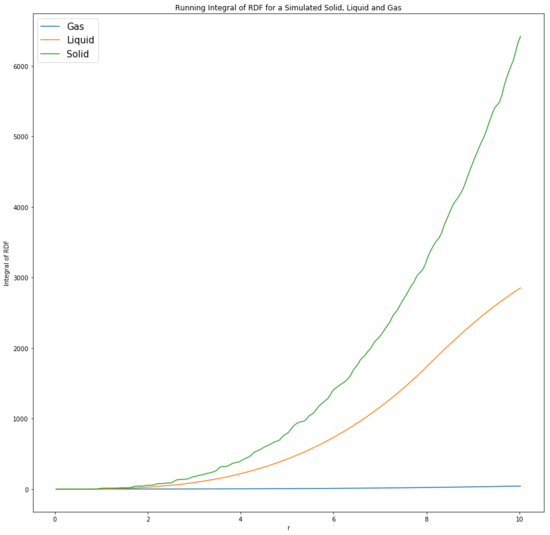
The radial distribution function (RDF) is the probability density of finding an atom in a certain position. Relative to a specific atom, the RDF can be used to determine the structure of the atomic arrangement and the coordination sphere of the particular atom. Tick The integral of the RDF gives the number of atoms found at the radial distance from the atom and indicates the degree of order. This is useful as it can determine the size of the lattice and other thermodynamic properties such as pressure and potential energy can be found from the plot.

The RDF for gas has a single broad peak due to the disordered structure. The peak is likely to be present at the equilibrium bond distance, hence giving a larger probability of encountering another particle.bond? Additionally, the peak is broad which may indicate the bond oscillation as the particles are not fixed. At a distance less than that, the RDF is zero due to particle repulsion as modelled via the Lennard-Jones potential and this occurs for all phases. The high energy motion of the gas particles ensures that the density of this phase is low and averaged over the fixed volume, with no long range order structure as indicated by the RDF value falling to 1 after a short distance. This highlights that beyond the equilibrium bond distance, the probability of finding a gas particle is constant regardless of distance due to the diffuse nature of the phase. Should the rdf be zero? what does it measure and how? Could also talk about dynamic averaging here.

In comparison, the liquid phase is slightly more ordered as illustrated by the additional two peaks, indicating more coordination shells.Tick The peaks are broad due to the dynamic nature of liquids and oscillate around the value of 1.Tick The decrease in probability below 1 could be due to intermolecular repulsion.Kind of... the troughs between peaks are because there isn't anything inbetween atomic neighbours However, since liquids are neither fixed into position like solids nor as diffuse as gas, they tend to align with other molecules (particularly in solvents) to generate a lower energy solvation shell giving rise to the presence of a short range ordered structure.

The peaks in the solid phase are sharp due to the rigidity of the structure as the particles are fixed in place and vibrate about their fixed position, hence why the probability of finding a particle in a certain position is high as they are held in a lattice. The lattice structure is regular, leading to a long range order for the solid.Tick, good The first three peaks are associated with the 3 closest neighbours, with the first peak being the adjacent particles. The fluctuations are due to the particles not being held too closely to reduce repulsion. Additionally, the integral of the RDF affirms that the solid is highly ordered, with the gas being the least ordered in confirmation of the theory. In a perfect crystal, the RDF would be a periodix series of sharp peaks, indicating the certainty in the atomic positions. Tick

The lattice spacing is the property of the crystal lattice and is the minimum distance between repeat lattices. For a face centred cubic lattice, the lattice spacing can be found by identifying the distance between the atom on one corner and the atom on the adjacent corner. The spacing is therefore 1.175. The coordination number is the quantity of particles immediately surrounding a certain particle. Tick

Lattice Coordination of Solid

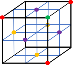
The particles outside of the first three coordination shells have been omitted from the diagram for ease of understanding. From the perspective of the green particle, the primary coordination shell is comprised of the lattice sites represented by the purple particles and correspond to the first peak. They are located in the centre of the adjacent faces to the green atom. The second peak corresponds to the lattice sites shown by red particles on the corners of the unit cell. Finally, the third coordination shell and peak is associated with the yellow particles located on the non-adjacent faces.

Peak	r	Integral	Coordination Number
1	0.975	8.77	12
2	1.175	12.00	6
3	1.675	30.27	24	Tick

Dynamical Properties and the Diffusion Coefficient

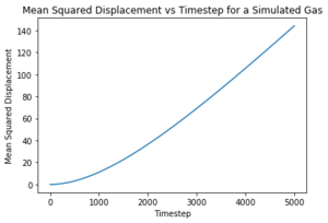
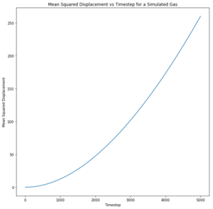
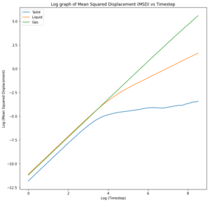
What ensemble are you using here? The Mean Squared Displacement (MSD) is the measure of the change in position of a particle from an initial position over time and is used to measure the diffusion coefficient $D$. Experimentally, the MSD can be measured in a photon light scattering experiment where lasers are used to scatter light to locate the position of particles. Tick

Mean Squared Distribution Plots (Simulated)

Gas	Liquid	Solid
Mean Squared Distribution for a Gas	Mean Squared Distribution for a Liquid	Mean Squared Distribution for a Solid

Log Graph for the Mean Squared Distribution plots against Temperature

Diffusion Coefficient

Phase	Simulated Data	One Million Atoms (Given)
Gas	1.16	0.974
Liquid	0.504	0.507
Solid	0.0005	0

Units?

The log plots illustrate the motion of the particles. Nice The motion of the particles in all phases are ballistic, that is, their distance from an initial position increases linearly with time and this can be seen for both sets of data. Nope, linearity is diffusive.. The solid particle motion plateaus over time due to energy loss whereas both the liquid and the vapour particles are able to travel through diffusion, unlike the liquid in a fixed position.

The diffusion coefficients calculated agree with the theory presented by the radial distribution functions. Due to the fixed lattice structure of solid, the particles are unable to move and thus unable to diffuse through space. They are limited to vibrating about their fixed position and have fewer degrees of freedom. Consequently, the diffusion coefficient in negligible and the simulation results agree with the data given for one million atoms. Increased temperature to increase the thermal energy would perhaps cause the particles to vibrate faster and faster until the critical temperature was reached to break the bonds and melt the solid at which point diffusion would occur. Tick

The liquid diffusion coefficients for both sets of data were also very similar. Liquids have more degrees of freedom than solid but are still constrained by the short range order as shown by the RDF. This means the liquids are able to diffuse but not as rapidly as gases. Gases are able to diffuse quickly as they possess all translational degrees of freedom.

Any discrepancies in data were due to the difference in size of data set. The values for one million atom are more likely to be accurate as the data was averaged over a larger set.

Mean Squared Distribution Plots (Simulated)

Gas	Liquid	Solid
Mean Squared Distribution for a Gas (one million atoms)	Mean Squared Distribution for a Liquid (one million atoms)	Mean Squared Distribution for a Solid (one million atoms)

Log Graph for the Mean Squared Distribution plots against Temperature (one million atoms)

Velocity Autocorrelation Function

Velocity Autocorrelation Function

Data Set	Liquid and Solid	Gas
Simulated Data	VCAF Plot vs Timestep for a solid and a liquid	VCAF Plot vs Timestep for a gas
One Million Atoms	VCAF Plot vs Timestep for a solid and a liquid (one million atoms)	VCAF Plot vs Timestep for a gas (one million atoms)

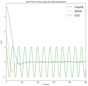
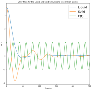
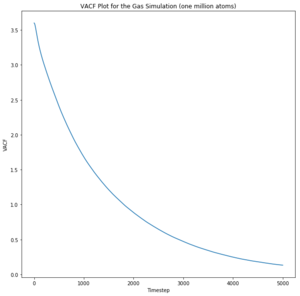
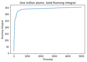
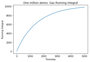
A 1D harmonic oscillator has been plotted on the VACF for comparison. The minima in the VACF for the liquid and solid system represent a negative correlation, suggesting that the velocity is negative and moving in the opposite direction to the initial velocity. Although the solid VACF does appear to oscillate, energy is lost quickly through interactions with neighbouring atoms and so velocity decreases until motion ceases and the solid oscillates no more; the oscillation is damped. This oscillatory behaviour is exhibited in a solid as the particles are able to oscillate around a fixed position. In the harmonic oscillator, total energy is conserved and so theoretically it would be able to oscillate indefinitely. This model displays a system where the particles do not interact and there is zero energy loss, indicating a perfect oscillator. Fundamentally, the trough represents collisions

The liquid appears to oscillate very briefly as given by the minima, illustrating that energy is lost very quickly to other particles through collision or other means. Additionally, the liquid particles are not fixed and do not oscillate in one position like a solid; they instead exhibit diffusive behaviour. This means that correlation decreases even faster than for the solid. Likewise, the gas particles exhibit random motion and diffusive behaviour and therefore do not correlate to the harmonic oscillator at all.

Velocity Autocorrelation Function Running Integrals

Data Set	Liquid	Solid	Gas
Simulated Data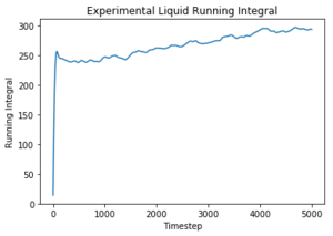
One Million Atoms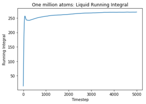

Diffusion Coefficient

Phase	Simulated Data	One Million Atoms (Given)
Gas	7.70	1.09
Liquid	0.098	0.090
Solid	0.0001	$4.54\times 10^{-5}$

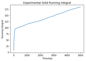
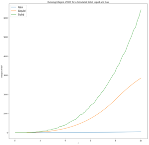
The diffusion coefficients follow the same trend as predicted in the mean squared displacement plots. However, the simulated data is quite different to the given data set for one million atoms and the MSD approximation, although they are on the same order of magnitude. The trapezium rule is only a rough approximation of the area under a graph and it is a likely source of error for the discrepancy of the values as it cannot map precisely to the curve of the plots. However, the values given for one million atoms were similar to those given by the MSD plots and therefore there must have been another error source. The running integrals for the liquid and gas do not appear to have converged and therefore give an smaller value for the diffusion coefficient; this could be rectified by continuing the VACF simulation for longer until a convergence in the integral was seen. The largest error is considered to be the difference in size of the set from which the data was taken. The one million atoms allow a more accurate average to be taken to account for any anomalous results. Tick, again units

Conclusion

Not bad, be careful not to go off on tangents and claim things that you don't see. Take your time and breathe- Not a bad conclusion though, make your claims, justify them and evidence them. Simulations of Lennard-Jones liquids, solids and vapours were successfully run on the LAMMPS application on the HPC supercomputer, analysed on the VMD programme and plotted on Python to examine how different thermodynamic properties varied. This was done by carrying out simulations to vary density with temperature under a npt ensemble, heat capacity against temperature for a nvt ensemble, calculating the radial distribution function to locate the lattice sites and determine structure of a solid, liquid and gas and approximate the diffusion coefficient with both the mean squared distribution and the velocity autocorrelation function to compare.

It was found that number density increased with pressure but was lower than ideal behaviour due to the Lennard-Jones parameters which allowed for repulsion between the particles. At higher temperatures, the simulation tended towards ideality as the particles were further apart and interacted less and hence for a given unit of volume, the density decreased. Moreover, at higher pressures the number density particles in a given area were greater than at a lower pressure and so interaction between the particles increased to deviate from the ideal gas law.

Heat capacity decreased as temperature increased; the increased thermal energy made it easier to raise the internal energy of the system and populate higher energy levels so the total energy of the system fluctuates less. Did it? Here we see that it's harder to heat a hot thing. A more dense system would have a larger number of particles in a given volume and so the thermal energy is more widely distributed and lower energy states are occupied, leading to a larger value for heat capacity. Peaks at 2.2 and 2.6 were hypothesised to have been due to a change in phase, during which heat capacity was infinite and temperature did not change.

The radial distribution function affirmed that solids had the most ordered structure. The solid RDF had sharp peaks that extended to a greater distance than liquid or gas. This corresponded to the solid vibrating around a fixed position in a coordinated lattice, giving an extended crystal structure. The gas RDF had a singular broad peak that dropped to 1 very quickly. This shows that the structure is disordered due to the diffuse nature of the gas. Liquids fell in between the two but maintain a short range coordination sphere and was slightly more ordered than gas indicated by the three broad peaks. Lattice spacing was found to be 1.175.

The diffusion coefficient for both the mean squared distribution (MSD) and velocity autocorrelation function (VACF) gave the diffusion coefficients: Gas = 1.16 (MSD), 7.70 (VACF); Liquid = 0.504 (MSD), 0.098 (VACF); Solid = 0.0005 (MSD), 0.0001 (VACF). The solid was correlated for longer as it did not have the external factor of diffusion as the liquid did. The minima in the plot corresponded to a change in direction to give a negative velocity (from the initial position).span style="color:red">the time taken for all particles to collide exactly once It was surmised that the VACF values were less accurate as the running integrals for gas and liquid did not converge and because the trapezium rule approximation could not be fitted exactly to the curves so would have given a smaller value than determined. However, the largest error was thought to be the discrepancy in the size of the data set between the simulated and given data. Should a larger population testing have been carried out, a more accurate average value could have been determined.

Tasks

The Velocity-Verlet Algorithm

Open the file HO.xls. In it, the velocity-Verlet algorithm is used to model the behaviour of a classical harmonic oscillator. Complete the three columns "ANALYTICAL", "ERROR", and "ENERGY": "ANALYTICAL" should contain the value of the classical solution for the position at time t, "ERROR" should contain the absolute difference between "ANALYTICAL" and the velocity-Verlet solution (i.e. ERROR should always be positive -- make sure you leave the half step rows blank!), and "ENERGY" should contain the total energy of the oscillator for the velocity-Verlet solution. Remember that the position of a classical harmonic oscillator is given by $x\left(t\right)=A\cos (\omega t+\varphi )$ (the values of $A$, $\omega$, and $\varphi$ are worked out for you in the sheet). For the default timestep value, 0.1, estimate the positions of the maxima in the ERROR column as a function of time. Make a plot showing these values as a function of time, and fit an appropriate function to the data. Experiment with different values of the timestep. What sort of a timestep do you need to use to ensure that the total energy does not change by more than 1% over the course of your "simulation"? Why do you think it is important to monitor the total energy of a physical system when modelling its behaviour numerically?

Comparing the Classical Harmonic Oscillator Solution to the Velocity-Verlet Algorithm

Solution Type	Plot
Analytical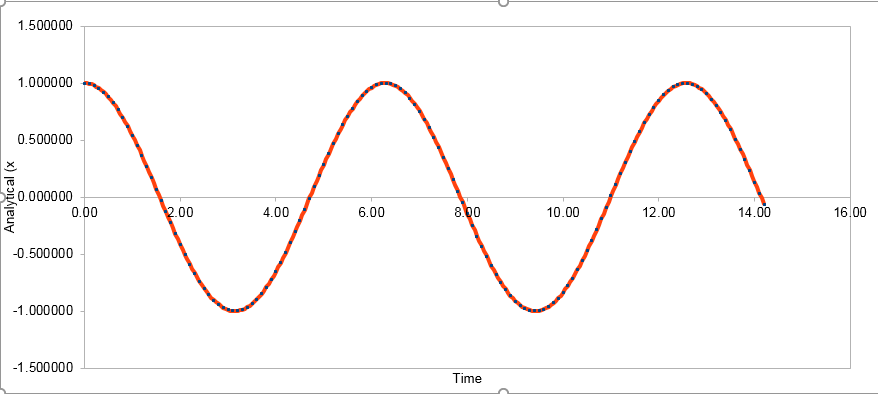
Energy
Error (Timestep 0.1)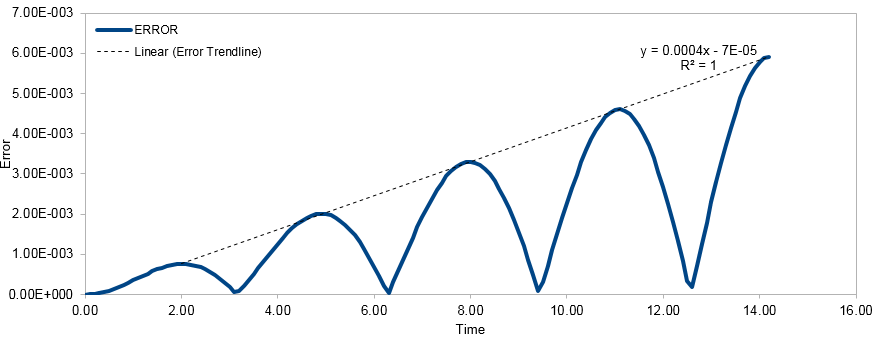

The energy of the system was given by the total of both the kinetic energy $\frac{1}{2}m{v}^2$ and potential energy $\frac{1}{2}k{x}^2$. A timestep of 0.2 or under ensures that the total energy of the simulation does not alter beyond 1%. As the simulations are run as isolated systems, total energy must be conserved. The Velocity-Verlet allows for fluctuations as the Taylor expansion is a very good approximation. However, fluctuations must be minimised as large variations of energy would produce inaccuracies in the measured thermodynamic properties of the system. Smaller timesteps give greater accuracy but may extend the time required to run the simulation. In this case, a timestep of 0.2 would give the desired results fastest. Tick, good

Atomic Forces

For a single Lennard-Jones interaction, $\varphi \left(r\right)=4ϵ(\frac{{\sigma }^{12}}{r^{12}}-\frac{{\sigma }^6}{r^6})$, find the separation, $r_0$, at which the potential energy is zero. What is the force at this separation? Find the equilibrium separation, $r_{eq}$, and work out the well depth $(\varphi \left(r_{eq}\right))$. Evaluate the integrals $\underset{2\sigma }{\overset{\mathrm{\infty }}{\int }}\varphi \left(r\right)\mathrm{d}r$, $\underset{2.5\sigma }{\overset{\mathrm{\infty }}{\int }}\varphi \left(r\right)\mathrm{d}r$, and $\underset{3\sigma }{\overset{\mathrm{\infty }}{\int }}\varphi \left(r\right)\mathrm{d}r$ when $\sigma =ϵ=1.0$.

For the separation $r_0$:

$\varphi \left(r\right)=4ϵ(\frac{{\sigma }^{12}}{r^{12}}-\frac{{\sigma }^6}{r^6})$

$\frac{{\sigma }^{12}}{r^{12}}-\frac{{\sigma }^6}{r^6}=0$

$\frac{{\sigma }^{12}}{r^{12}}=\frac{{\sigma }^6}{r^6}$

$\frac{{\sigma }^6}{r^6}=1$

${\sigma }^6=r^6$

$r_0=\sigma$

Tick, good

The force at $r_0$:

$F=-\frac{\varphi (r)}{dr}$

$=-4ϵ(\frac{-12{\sigma }^{12}}{r^{13}}+\frac{6{\sigma }^6}{r^7})$

Tick, good

when $r_0=\sigma$:

$F=4ϵ(\frac{12}{\sigma }-\frac{6}{\sigma })$

$=4ϵ\left(\frac{6}{\sigma }\right)$

$=\frac{24ϵ}{\sigma }$

Tick, good

The equilibrium separation, $r_{eq}$, is given by finding the minimum:

$\frac{\varphi (r)}{dr}=4ϵ(\frac{-12{\sigma }^{12}}{r^{13}}+\frac{6{\sigma }^6}{r^7})=0$

$\frac{12{\sigma }^{12}}{r^{13}}=\frac{6{\sigma }^6}{r^7}$

$2{\sigma }^6=r^6$

$r_{eq}=2^{1/6}\sigma$

Tick, good

Well depth:

$\frac{\varphi (r)}{dr}=4ϵ(\frac{{\sigma }^{12}}{(2^{1/6}\sigma {)}^{12}}-\frac{{\sigma }^6}{(2^{1/6}\sigma {)}^6})$

$=4ϵ(\frac{{\sigma }^{12}}{4{\sigma }^{12}}-\frac{{\sigma }^6}{2{\sigma }^6})$

$=ϵ=2ϵ=-ϵ$

Tick, good

Integrals when $\sigma =ϵ=1.0$:

$\underset{2\sigma }{\overset{\mathrm{\infty }}{\int }}\varphi \left(r\right)\mathrm{d}r=4ϵ\underset{2\sigma }{\overset{\mathrm{\infty }}{\int }}(\frac{{\sigma }^{12}}{r^{12}}-\frac{{\sigma }^6}{r^6})\mathrm{d}r$

$=4ϵ[\frac{{\sigma }^{12}}{-11r^{11}}+\frac{{\sigma }^6}{5r^5}{]}_{2\sigma }^{\mathrm{\infty }}$

$=-0.0248$

Tick, good

$\underset{2.5\sigma }{\overset{\mathrm{\infty }}{\int }}4ϵ(\frac{{\sigma }^{12}}{r^{12}}-\frac{{\sigma }^6}{r^6})dr$

$=4ϵ{[-\frac{1}{11}\frac{{\sigma }^{12}}{r^{11}}+\frac{1}{5}\frac{{\sigma }^6}{r^5}]}_{2.5\sigma }^{\mathrm{\infty }}$

$=-8.18\times 10^{-3}$

Tick, good

$\underset{3\sigma }{\overset{\mathrm{\infty }}{\int }}4ϵ(\frac{{\sigma }^{12}}{r^{12}}-\frac{{\sigma }^6}{r^6})dr$

$=4ϵ{[-\frac{1}{11}\frac{{\sigma }^{12}}{r^{11}}+\frac{1}{5}\frac{{\sigma }^6}{r^5}]}_{2.5\sigma }^{\mathrm{\infty }}$

$=-3.29\times 10^{-3}$

Tick, good

Estimate the number of water molecules in 1ml of water under standard conditions. Estimate the volume of 10000 water molecules under standard conditions.

Assuming a density of 1g per ml then

$moles=\frac{mass}{Mr}$

,

$$\begin{gathered} N=\frac{mass\times N_a}{M_r}=\frac{1\times 6.022\times 10^{23}}{18.0}=3.35\times 10^{22} \\ molecules \end{gathered}$$

Tick, good

$Density=\frac{mass}{volume}$

so

$$\begin{gathered} \frac{1\times 10^4\times 18.0}{6.022\times 10^{23}}=2.989\times 10^{-19} \\ g \end{gathered}$$

Tick, good

$$\begin{gathered} V=\frac{mass}{density}=\frac{2.989\times 10^{-19}}{1}=2.989\times 10^{-19} \\ c{m}^3=2.989\times 10^{-25} \\ {m}^3 \end{gathered}$$

Tick, good

Consider an atom at position $(0.5,0.5,0.5)$ in a cubic simulation box which runs from $(0,0,0)$ to $(1,1,1)$. In a single timestep, it moves along the vector $(0.7,0.6,0.2)$. At what point does it end up, after the periodic boundary conditions have been applied? After the boundary conditions, the atom is at

$(0.2i+0.1j+0.7k)$

Tick, good

This is because the constraints cause the atoms to pass through one side of the cubic simulation box and emerge at the other side.

The Lennard-Jones parameters for argon are $\sigma =0.34\mathrm{n}\mathrm{m}$, $$\begin{gathered} ϵ \\ / \\ {k}_B=120\mathrm{K} \end{gathered}$$. If the LJ cutoff is $r^{*}=3.2$, what is it in real units? What is the well depth in $$\begin{gathered} {\mathrm{k}\mathrm{J} \\ \mathrm{m}\mathrm{o}\mathrm{l}}^{-1} \end{gathered}$$? What is the reduced temperature $T^{*}=1.5$ in real units?

$r^{*}=\frac{r}{\sigma }=3.2$

$$\begin{gathered} r=3.2\sigma =3.2\times 0.34\times 10^{-19}=1.088\times 10^{-9}=1.088 \\ nm \end{gathered}$$

Tick, good

$T^{*}=\frac{k_{b}T}{ϵ}=1.5$

Tick, good

$$\begin{gathered} T=\frac{1.5ϵ}{k_b}=1.5\times 120=180 \\ K \end{gathered}$$

Tick, good

$$\begin{gathered} Well \\ Depth=\varphi (r_{eq})=-ϵ=-120\times 1.381\times 10^{-}23 \\ J=-1.66\times 10^{-24}kJ=-0.998 \\ kJ \\ mo{l}^{-1} \end{gathered}$$

Tick, good

Equilibration

Why do you think giving atoms random starting coordinates causes problems in simulations? Hint: what happens if two atoms happen to be generated close together?

Should two atoms be generated close together when each atom is assigned random starting coordinates, the simulation may be inaccurate due to the interaction of the atoms. The two atoms may repel strongly and in doing so, disrupt the dynamics of the system by distorting the behaviour of the neighbouring atoms. However, if the interaction between the atoms are favourableand the distance between them is within the Van der Waals radius then a bond will be approximated between them. The molecule may then interact differently with the other free atoms in the system. Tick

Satisfy yourself that this lattice spacing corresponds to a number density of lattice points of 0.8. Consider instead a face-centred cubic lattice with a lattice point number density of 1.2. What is the side length of the cubic unit cell?

Lattice points are present on each corner of the simple cubic lattice unit cell, so the distance between the lattice points is 1.07722 (reduced units) given that:

Lattice spacing in x,y,z = 1.07722 1.07722 1.07722

Since a simple cubic lattice contains one lattice point per unit cell, $NumberDensity=\frac{1}{volume}=\frac{1}{(1.07722{)}^3}=0.8$ Tick

For a face centred cubic lattice, there are 4 lattice points in the unit cell. Therefore, if number density = 1.2 The side length of the unit cell $l$:

$l=\sqrt[3]{(}\frac{4}{1.2})=1.4938$Tick

Consider again the face-centred cubic lattice from the previous task. How many atoms would be created by the create_atoms command if you had defined that lattice instead?

As the FCC lattice has 4 lattice points per unit cell, a 10x10x10 box contains 1000 unit cells and therefore 4000 atoms are created in the box. Tick

Using the LAMMPS manual , find the purpose of the following commands in the input script:

Mass I Value: 'The Mass I Value command determines the mass for one or more atom types. The I index can be specified in one of two ways. An explicit numeric value can be used, as in the 1st example above. Or a wild-card asterisk can be used to set the mass for multiple atom types. This takes the form “*” or “*n” or “n*” or “m*n”. If N = the number of atom types, then an asterisk with no numeric values means all types from 1 to N. A leading asterisk means all types from 1 to n (inclusive). A trailing asterisk means all types from n to N (inclusive). A middle asterisk means all types from m to n (inclusive).'

Pair_style lj/cut/opt: 'During initialisation, there are set parameters that need to be defined before atoms are created or read-in from a file. If there are fore-field parameters present in the files to be read then the pair_style command determines the Lennard-Jones Potential for the force field. It is the formula used by the LAMMPS programme to compute pairwise interactions. The pair potentials are defined between atom pairs within a certain cutoff distance and the set of active interactions typically changes over time.'

The lj/cut styles compute the standard 12/6 Lennard-Jones potential, given by

$E=4ϵ\left[\right(\frac{\sigma }{r}{)}^{12}-\left(\frac{\sigma }{r}{)}^6\right]$ $r<r_c$

$r_c$ 'is the cutoff, after which the interaction is assumed to be zero as the particles are too far apart.'

Here the first term describes the repulsive forces between the particles and the second terms gives the attractive forces.

$E$ is the intermolecular potential between the two atoms.

$ϵ$ is the depth of the potential well and indicates the strength of the particle attraction.

$\sigma$ is the distance when E=0, the Van der Waals radius. It is half the internuclear distance between two non-bonding particles.Tick

$r$ is the distance between the two atoms measured from the centre of each atom.

Pair_coeff I J args: 'I,J = atom types (see asterisk form below) args = coefficients for one or more pairs of atom types.The command specifies the pairwise force field coefficients for one or more pairs of atom types. The number and meaning of the coefficients depends on the pair style. Pair coefficients can also be set in the data file read by the read_data command or in a restart file. LAMMPS sets the coefficients for the symmetric J,I interaction to the same values.

Given that we are specifying ${\mathbf{x}}_i\left(0\right)$ and ${\mathbf{v}}_i\left(0\right)$, which integration algorithm are we going to use?

Given that the initial conditions require the position and velocity to be set to zero at the same time, it is assumed that the acceleration depends only on position and not velocity. In this case, it is appropriate for the Velocity-Verlet Algorithm to be used. A Taylor expansion is used to determine the atomic velocities and position of the atoms, through which both the acceleration and forces acting on the atoms can be found. Tick

The second line (starting "variable timestep...") tells LAMMPS that if it encounters the text ${timestep} on a subsequent line, it should replace it by the value given. In this case, the value ${timestep}is always replaced by 0.001. In light of this, what do you think the purpose of these lines is?

The variable timestep command is used in lieu of 'timestep' as it allows different values to be changed easily without having to repeat the command several times.

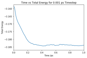
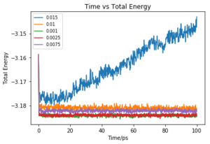
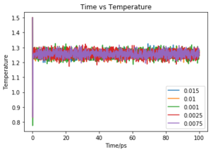
Make plots of the energy, temperature, and pressure, against time for the 0.001 timestep experiment (attach a picture to your report). Does the simulation reach equilibrium? How long does this take? When you have done this, make a single plot which shows the energy versus time for all of the timesteps (again, attach a picture to your report). Choosing a timestep is a balancing act: the shorter the timestep, the more accurately the results of your simulation will reflect the physical reality; short timesteps, however, mean that the same number of simulation steps cover a shorter amount of actual time, and this is very unhelpful if the process you want to study requires observation over a long time. Of the five timesteps that you used, which is the largest to give acceptable results? Which one of the five is a particularly bad choice? Why? The simulation reaches equilibrium at ~0.2 ps as shown in Fig.1. The plot indicates that the simulation converge to its lowest possible energy and remained at that energy. As the pressure and temperature are a constant average value, the simulation is working.

Fig.1 The convergence of total energy indicating that the simulation reached equilibrium at ~0.2 ps

Fig.2 Total Energy vs Time for a 0.001 ps Timestep

Fig.3 Total Energy vs Pressure for a 0.001 ps Timestep

Fig.4 Total Energy vs Temperature for a 0.001 ps Timestep

Of the 5 timesteps, the largest timestep to give a useful value is 0.01 ps as the energy still converges and would have done so first before any smaller time steps (Fig. 5). However, the 0.015 ps timestep cannot be used as not only does the energy not converge but actually increases. Due to the large timestep, a limited number of values were taken and the abrupt changes of the results were interpreted as high energy and so the energy of the system does not converge. This simulation is therefore not useful. Tick

Fig.5 The convergence of total energy for all 5 timesteps in ps

Fig.6 Total Energy vs Temperature for all timesteps

Fig.7 Total Energy vs Pressure for all timesteps

Running Simulations Under Specific Conditions

Choose 5 temperatures (above the critical temperature T^* = 1.5), and two pressures (you can get a good idea of what a reasonable pressure is in Lennard-Jones units by looking at the average pressure of your simulations from the last section). This gives ten phase points — five temperatures at each pressure. Create 10 copies of npt.in, and modify each to run a simulation at one of your chosen \left(p, T\right) points. You should be able to use the results of the previous section to choose a timestep. Submit these ten jobs to the HPC portal. While you wait for them to finish, you should read the next section.

The pressures chosen were 2.5 and 3.5. The temperatures: 2.0, 5.0, 7.5, 9.0. 10.0 with a timestep of 0.001.

We need to choose $\gamma$ so that the temperature is correct $T=\mathfrak{𝔗}$ if we multiply every velocity $\gamma$. We can write two equations:

$\frac{1}{2}\sum _i{m}_i{v}_i^2=\frac{3}{2}N{k}_{B}T$

$\frac{1}{2}\sum _i{m}_i{\left(\gamma v_i\right)}^2=\frac{3}{2}N{k}_B\mathfrak{𝔗}$

$T=\frac{\sum _i{m}_i{v}_i^2}{3N{k}_b}$

$\mathfrak{𝔗}=\frac{\sum _i{m}_i{\left(\gamma v_i\right)}^2}{3N{k}_b}={\gamma }^2\frac{\sum _i{m}_i{v}_i^2}{3N{k}_b}$

$\mathfrak{𝔗}={\gamma }^{2}T$

${\gamma }^2=\frac{\mathfrak{𝔗}}{T}$

$\gamma =\sqrt{\frac{\mathfrak{𝔗}}{T}}$

Tick, nice

Use the manual page to find out the importance of the three numbers 100 1000 100000. How often will values of the temperature, etc., be sampled for the average? How many measurements contribute to the average? Looking to the following line, how much time will you simulate?

Every 100 timesteps, input values are sampled. An average is calculated over a sample size of 1000 input values (taken every 100 timesteps) and after each average taken there are 100000 steps before the next one is taken. The amount of time simulated was 100 units found by multiplying the number of steps (100000) by timestep (0.001). Tick

Plotting the Equations of State

When your simulations have finished, download the log files as before. At the end of the log file, LAMMPS will output the values and errors for the pressure, temperature, and density $\left(\frac{N}{V}\right)$. Use software of your choice to plot the density as a function of temperature for both of the pressures that you simulated. Your graph(s) should include error bars in both the x and y directions. You should also include a line corresponding to the density predicted by the ideal gas law at that pressure. Is your simulated density lower or higher? Justify this. Does the discrepancy increase or decrease with pressure?

Fig.5 Pressure=2.5

Fig.6 Pressure=3.5

Simulated density is lower than expected. This discrepancy is due to the assumptions for a perfect gas: zero interactions with other particles, particles modelled as points and Lennard-Jones-parameters a and b to be zero. As the simulated particles are assumed to interact, the discrepancies become more apparent with greater interaction. At higher temperatures, the simulation tends towards ideality as the particles are further apart and interact less. Moreover, at higher pressures the number density particles in a given area is greater than at a lower pressure and so interaction increases, tending further from ideality.

Heat Capacity Calculation

As in the last section, you need to run simulations at ten phase points. In this section, we will be in density-temperature $({\rho }^{*},T^{*})$ phase space, rather than pressure-temperature phase space. The two densities required at 0.2 and 0.8, and the temperature range is 2.0, 2.2, 2.4, 2.6, 2.8. Plot $C_V/V$ as a function of temperature, where V is the volume of the simulation cell, for both of your densities (on the same graph). Is the trend the one you would expect? Attach an example of one of your input scripts to your report.

Fig.8 The input file for number density=0.2 and T=2.0 to calculate heat capacity

Fig.9 Plot for heat capacity/volume against temperature for number density=0.2

Fig.10 Plot for heat capacity/volume against temperature for number density=0.8

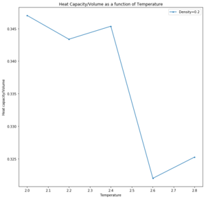
This simulation was run as a simple cubic lattice structure due to the temperatures being above the critical temperature and are therefore assumed to be fluids. The trend is expected as heat capacity decreases with temperature increase as it is easier to populate higher energy levels and total energy of the system fluctuates less. A more dense system has a larger number of particles in a given volume and so the thermal energy is more widely distributed. Lower energy states are occupied. The anomaly is hypothetically due to a change in phase, to another liquid or vapour phase, upon which the heat capacity is infinite and temperature does not change.

Radial Distribution Function

Perform simulations of the Lennard-Jones system in the three phases. When each is complete, download the trajectory and calculate $g(r)$ and $\int g(r)\mathrm{d}r$. Plot the RDFs for the three systems on the same axes, and attach a copy to your report. Discuss qualitatively the differences between the three RDFs, and what this tells you about the structure of the system in each phase. In the solid case, illustrate which lattice sites the first three peaks correspond to. What is the lattice spacing? What is the coordination number for each of the first three peaks?

Radial Distribution Function for the Simulated Solid, Liquid and Gas

Integral of the Radial Distribution Function

The gas RDF has a singular broad peak that drops to 1 very quickly. This shows that the structure is disordered due to the diffuse nature of the gas. The density is averaged over the fixed volume. It is suggested that the peak is broad due to the oscillation of a possible bond.

The liquid RDF is less diffuse than the gas and has a slightly more ordered structure. Liquids are dynamic and not fixed in position like solid are. They can therefore rearrange and align to form coordination spheres of lower energy (like when being solvated). There are 3 broad peaks indicating 3 coordination shells but drop to RDF of 1 after that, suggesting no long range structure

The solid RDF has sharp peaks that extend for a long distance. This corresponds to the solids vibrating around a fixed position in a coordinated lattice, giving an extended crystal structure.

The lattice spacing is the minimum distance between lattices = 1.175.

Peak	r	Integral	Coordination Number
1	0.975	8.77	12
2	1.175	12.00	6
3	1.675	30.27	24

Dynamical Properties and the Diffusion Coefficient

In the D subfolder, there is a file liq.in that will run a simulation at specified density and temperature to calculate the mean squared displacement and velocity autocorrelation function of your system. Run one of these simulations for a vapour, liquid, and solid. You have also been given some simulated data from much larger systems (approximately one million atoms). You will need these files later.

Mean Squared Distribution Plots (Simulated)

Gas	Liquid	Solid
Mean Squared Distribution for a Gas	Mean Squared Distribution for a Liquid	Mean Squared Distribution for a Solid

Log Graph for the Mean Squared Distribution plots against Temperature

Phase	Simulated Data	One Million Atoms (Given)
Gas	1.16	0.974
Liquid	0.504	0.507
Solid	0.0005	0

Mean Squared Distribution Plots (One Million Atoms)

Gas	Liquid	Solid
Fig.16 Mean Squared Distribution for a Gas (one million atoms)	Fig.17 Mean Squared Distribution for a Liquid (one million atoms)	Fig.18 Mean Squared Distribution for a Solid (one million atoms)

Fig.19 Log Graph for the Mean Squared Distribution plots against Temperature (one million atoms)

Velocity Autocorrelation Function

In the theoretical section at the beginning, the equation for the evolution of the position of a 1D harmonic oscillator as a function of time was given. Using this, evaluate the normalised velocity autocorrelation function for a 1D harmonic oscillator (it is analytic!):

$C\left(\tau \right)=\frac{\underset{-\mathrm{\infty }}{\overset{\mathrm{\infty }}{\int }}v\left(t\right)v(t+\tau )\mathrm{d}t}{\underset{-\mathrm{\infty }}{\overset{\mathrm{\infty }}{\int }}{v}^2\left(t\right)\mathrm{d}t}$

$\underset{-\mathrm{\infty }}{\overset{\mathrm{\infty }}{\int }}\frac{A^2{\omega }^{2}sin(\omega t+\varphi )sin(\omega t+\omega \tau +\varphi )}{A^2{\omega }^{2}sin(\omega t+\varphi )}dt$

$=\underset{-\mathrm{\infty }}{\overset{\mathrm{\infty }}{\int }}\frac{\frac{1}{2}[cos(-\omega \tau )-cos(2\omega t+\omega \tau +2\varphi )]}{\frac{1}{2}[1-cos(2\omega t+2\varphi )]}dt$

$=[\frac{tcos(-\omega \tau )-sin(2\omega t+\omega \tau +2\varphi )(\frac{1}{2\omega })}{t-sin(2\omega t+2\varphi )(\frac{1}{2\omega })}{]}_{-\mathrm{\infty }}^{\mathrm{\infty }}$

$=[\frac{cos(-\omega \tau )-(\frac{1}{2\omega t})sin(2\omega t+\omega \tau +2\varphi )}{1-(\frac{1}{2\omega t})sin(2\omega t+2\varphi )}{]}_{-\mathrm{\infty }}^{\mathrm{\infty }}$

$=\frac{cos(-\omega \tau )-0}{1-0}$

$=cos(\omega \tau )$

Be sure to show your working in your writeup. On the same graph, with x range 0 to 500, plot $C\left(\tau \right)$ with $\omega =1/2\pi$ and the VACFs from your liquid and solid simulations. What do the minima in the VACFs for the liquid and solid system represent? Discuss the origin of the differences between the liquid and solid VACFs. The harmonic oscillator VACF is very different to the Lennard Jones solid and liquid. Why is this? Attach a copy of your plot to your writeup.

The harmonic oscillator differs as it represents an isolated system where total energy is conserved. This does not occur in the liquid or solid simulations as they interact with neighbouring particles and thus their oscillation is damped. The solid is correlated for longer as it does not have the external factor of diffusion as liquids do as solids remain in a fixed position. The minima correspond to a change in direction to give a negative velocity (from the initial position).

Velocity Autocorrelation Function

Data Set	Liquid and Solid	Gas
Simulated Data	VCAF Plot vs Timestep for a solid and a liquid	VCAF Plot vs Timestep for a gas
One Million Atoms	VCAF Plot vs Timestep for a solid and a liquid (one million atoms)	VCAF Plot vs Timestep for a gas (one million atoms)

Use the trapezium rule to approximate the integral under the velocity autocorrelation function for the solid, liquid, and gas, and use these values to estimate D in each case. You should make a plot of the running integral in each case. Are they as you expect? Repeat this procedure for the VACF data that you were given from the one million atom simulations. What do you think is the largest source of error in your estimates of D from the VACF?

The diffusion coefficients follow the expected trend as predicted with the MSD plot and are on the same order of magnitude. The values differ greatly between the smaller and larger data set and this could be due the smaller data set being unable to discount for any anomalies as the larger data set can be averaged more effectively to give a more accurate value. The trapezium rule is only an approximation as it cannot fit perfectly to the curve. The answer given will always fall short of the true answer. Additionally, the data had not yet converged for the running integral so the values for the gas and liquid were expected to be much larger.

Velocity Autocorrelation Function Running Integrals

Data Set	Liquid	Solid	Gas
Simulated Data
One Million Atoms

Diffusion Coefficient

Phase	Simulated Data	One Million Atoms (Given)
Gas	7.70	1.09
Liquid	0.098	0.090
Solid	0.0001	$4.54\times 10^{-5}$

References

- ↑ Sigala. P, Ruben, A, Liu.C, Determination of Hydrogen Bond Structure in Water versus Aprotic Environments To Test the Relationship Between Length and Stability, J. Am. Chem. Soc., 2015, 137 (17), 5730–5740
- ↑ Macdonald, D.D; Owen, D, Transport Numbers for Hydrochloric Acid at Elevated Temperatures, Can. J. Chem, 1972, 51, 2747.
- ↑ https://www.nist.gov/sites/default/files/documents/srd/NISTIR5078-Tab3.pdf 25/10/17
- ↑ Wong. K, Thermodynamics for Engineers, CRC Press, 2002, 269
- ↑ Chen. J, Yoo. C, High density amorphous ice at room temperature, PNAS, 108 (19), 2011, 7687
- ↑ Third Year Liquid Simulation Script, Robotham. O, Bresme. F, https://wiki.ch.ic.ac.uk/wiki/index.php?title=Third_year_simulation_experiment/Calculating_heat_capacities_using_statistical_physics 25/10/17
- ↑ Atkins. P; J, de Paula, Atkins’ Physical Chemistry, Oxford University Press, UK 10th edn., 2012, 861.
- ↑ Frenkel, Daan; Smit, Berend, Understanding molecular simulation from algorithms to applications, San Diego: Academic Press, Edn 2, 2002.
- ↑ Atkins. P; J, de Paula, Atkins’ Physical Chemistry, Oxford University Press, UK 10th edn., 2012, 681
- ↑ Berne, B.J.; Pecora, R. Dynamic Light Scattering. Courier Dover Publications, 2000, 412
- ↑ Salje. E, Physical Properties and Thermodynamic Behaviour of Minerals, D. Reidel Publishing Company, 1988, 511
- ↑ http://lammps.sandia.gov/doc/Section_commands.html#cmd_5 25/10/17