Talk:SZ3614ls

JC: General comments: All tasks attempted, but some mistakes and your written answers and explanations lack quite a lot of detail. Try to be more specific and focused in your answers to show that you understand the background theory.

Running Simulation

• Using HPC system to perform input scripts which have different timesteps
• The timesteps are 0.001, 0.0025, 0.0075, 0.01 and 0.015

Molecular dynamic simulation

Task

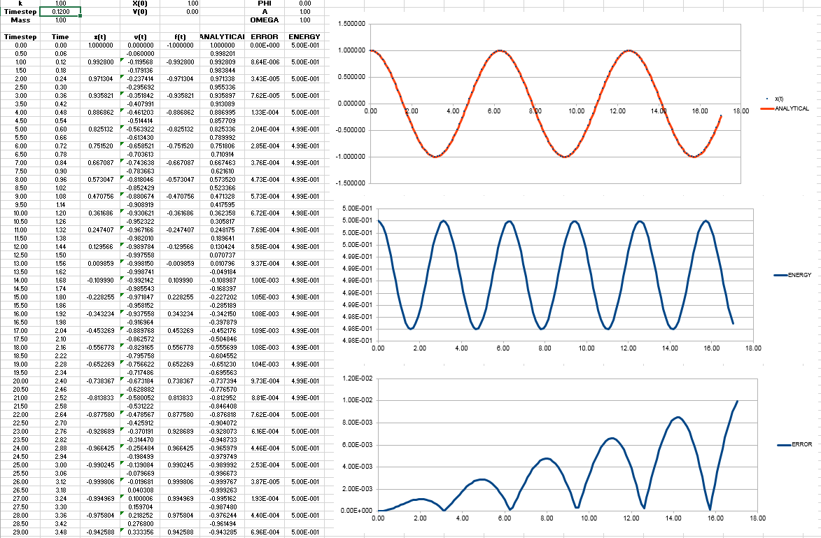
• complete column ANALYTICAL, ERROR, and ENERGY

ANALYTICAL is calculated by the classical harmonic oscillator equation. The position of a classical harmonic oscillator is $x\left(t\right)=A\cos (\omega t+\varphi )$${\left(1\right)}^{}$

ANALYTICAL vs time graph obtained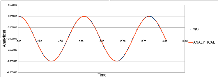

ERROR is the absolute value of the difference of ANALYTICAL and x(t). x(t) is already given in the file.

ERROR vs time graph is obtained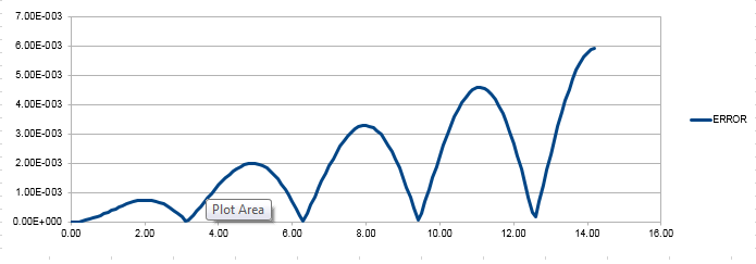

ENERGY is the total energy of the oscillator, $E_p+E_k=E_{total}$${\left(3\right)}^{}$, which is the sum of kinetic energy $E_k=\frac{1}{2}m{v}^2$ and the potential energy $E_p=\frac{1}{2}k{x}^2$

Energy vs time graph is obtained

JC: Why does the error oscillate?

Task

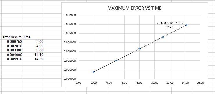
• find a graph of maxima ERROR vs time

As shown in the graph below the appropriate function is y=0.0004x-0.00007 the graph is obtained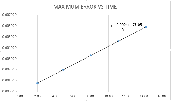

Task

• the timestep to ensure total energy changes not more than 1%

When the timestep is changed to 0.12, the total energy change is not more than 1%. Because the minimum and maximum on the energy graph is still within 1% from the middle value of the energy.

The energy vs time graph when timestep=0.12 is obtained

Task

• Find the separation, the force at this separation, the equilibrium separation, the well depth and the evaluate several integrals.

The separation $r_0$ = σ when the potential energy is 0, via L-J potential equation$\varphi \left(r\right)=4ϵ(\frac{{\sigma }^{12}}{r^{12}}-\frac{{\sigma }^6}{r^6})=0$${\left(2\right)}^{}$

thus $\frac{{\sigma }^6}{r^6}=1$

thus $r_0$ = σ

The force at this separation is 0 because the potential energy is 0 with the equation ${\mathbf{F}}_i=-\frac{\mathrm{d}U\left({\mathbf{r}}^N\right)}{\mathrm{d}{\mathbf{r}}_i}$${\left(2\right)}^{}$

JC: The force is not zero at sigma, it should be 24*epsilon/sigma. Look at a plot of the Lennard-Jones potential, the gradient is not 0 when the potential goes through zero.

The equilibrium separation is when the L-J potential is at the minimum.

Thus differentiation of L-J potential curve at this point should be equal to zero

Thus $\frac{\partial \varphi \left(r\right)}{\partial r}$=0

Then $4\epsilon ({\sigma }^{12}{r}^{-12}-{\sigma }^6{r}^{-6})$=0

Therefore $r=\sqrt[6]{2}\sigma$

JC: Correct answer, but the differentiation in the line above is wrong.

The well depth is the potential well, at the equilibrium, the well depth is -\varepsilon , calculated by substitute $r=\sqrt[6]{2}\sigma$ back into $\varphi \left(r\right)=4ϵ(\frac{{\sigma }^{12}}{r^{12}}-\frac{{\sigma }^6}{r^6})$

The integrals $\underset{2\sigma }{\overset{\mathrm{\infty }}{\int }}\varphi \left(r\right)\mathrm{d}r$=-0.02482, $\underset{2.5\sigma }{\overset{\mathrm{\infty }}{\int }}\varphi \left(r\right)\mathrm{d}r$=$-8.177\times 10^{-3}$, and $\underset{3\sigma }{\overset{\mathrm{\infty }}{\int }}\varphi \left(r\right)\mathrm{d}r$ =$-3.2901\times 10^{-3}$ when $\sigma =ϵ=1.0$.

JC: Show more of the working for the maths.

Task

• no. of water molecule in 1 ml water and volume of 10000 water molecules under under standard conditions.

The number of water molecule is $3.346\times 10^{22}$, via mass/volume equation and Avogadro's number with the calculation $1÷18\times 6.022\times 10^{23}$= $3.346\times 10^{22}$

The volume is $2.99\times 10^{-19}$ with the calculation $10000÷(6.022\times 10^{23})\times 18$=$2.99\times 10^{-19}$

JC: Correct.

Task

• After boundary condition, the point where it ends up at

It first goes to (1.2, 1.1, 0.7). As the atom goes outside the box, there is another stom goes in the box.

The end up point is (0.2, 0.1, 0.7).

JC: Correct.

Task

• The real unit of distance and temperature. the well depth value.

the real r=1.088 m ($r=r^{*}\times \sigma =3.2\times 0.34=1.088$)and the real T= 180 K ($T=T^{*}\times \frac{ϵ}{k_B}=1.5\times 120=180K$), via the L-J parameters Well depth Ԑ in $kJmo{l}^{-1}$ $$\begin{gathered} ϵ \\ / \\ {k}_B=120\mathrm{K} \end{gathered}$$ with Boltzmann's constant is approximately $1.3807\times 10^{-23}$ joules per kelvin${\left(10\right)}^{}$

thus Ԑ = $2.75\times 10^{-48}$ $$\begin{gathered} {\mathrm{k}\mathrm{J} \\ \mathrm{m}\mathrm{o}\mathrm{l}}^{-1} \end{gathered}$$

JC: The values for r and T are correct, but the well depth should be 0.997 kJ mol-1, you need to multiply by Avagadro's number.

Equilibration

Task

• Why random starting coordinates causes problem.

As two atoms get closer because of the attraction, they lose potential energy which is lost as heat. ${\left(3\right)}^{}$ The computational technique cannot simulate a system with the infinite potential because the atoms are going to blow up with the infinite potential.

JC: If particles are placed very close together the large repulsion force will make the simulation unstable and cause it to crash.

Task

• for ffc lattice, with lattice point number density 1.2, find the side length of the cubic unit cell

The ffc has four lattice point per one unit cell. Therefore the side length should be $\sqrt[3]{4÷1.2}$ = 1.494

Task

• The number of atoms created for ffc lattice via command

the command create_atom is to create 1 box which is 1000 unit cells. The ffc has four atoms per unit cell. Therefore, 4000 atoms would be created.

JC: Correct.

Task

• find the purpose of some commands

mass 1 1.0: 1 means the atome type is 1, 1.0 means the mass is 1.0 ${\left(4\right)}^{}$

pair_style lj/cut 3.0: lj/cut is the style, 3.0 is the argument. According to the L-J potential graph, cut-off value usually at a distance of 2.5.${\left(4\right)}^{}$

pair_coeff * * 1.0 1.0: ** sets the coefficients for all I J pairs, 1.0 is the argument which is the coefficient for one or more pairs of atom types ${\left(4\right)}^{}$

JC: What are the coefficients for a Lennard-Jones system and why is a cut off used?

Task

• ${\left(1\right)}^{}$

Use the variable instead just use the number, which allows us to change the variable efficiently. In a script, the variable will occur several times. If we want to change the variable value, we can simple change it at the second line instead of changing it several times in a scrpt.

JC: Correct.

Task

• plots of energy, temperature and pressure against time. equilibrium(how long to reach). plot of energy vs time. find a good timestep.

The plot of energy, temperature, pressure against time for 0.001 timestep is obtained.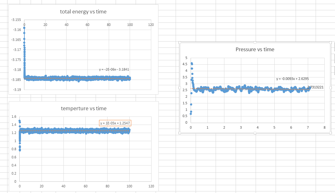 The simulation reached equilibrium as the constant energy, temperature, and pressure have obtained with a little bit fluctuation.It takes 0.39s for energy, 0.95s for temperature, 2.24s for pressure.

The plot of energy vs time for all timestep is obtained.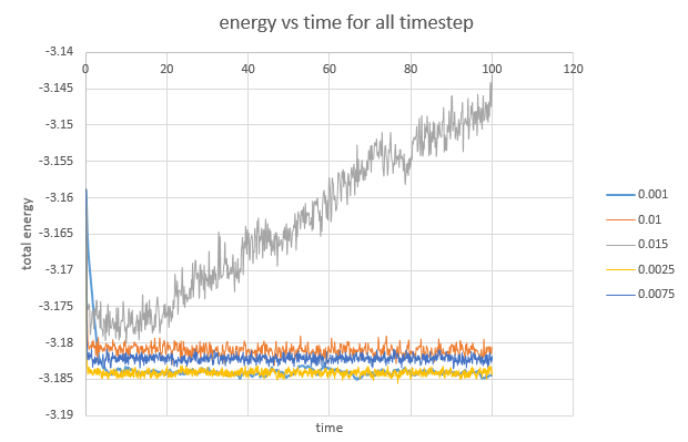

The largest timestep to give acceptable results is 0.01 because the simulation still reaches equilibrium even though very scattered graph.

The 0.015 timestep gives bad results. The slope of the energy vs time graph is too large and the simulation does not reach equilibrium

JC: Should the total energy depend on the choice of timestep? The largest timestep in which the total energy is unchanged compared to smaller timesteps is 0.025, this might be a better choice.

Simulation with specific conditions

Task

• choose five temperatures and two pressures

pressure: 2.65, 2.80 ( with the average pressure of simulations when the timestep is 0.001 as a basic idea)

Temperature: 1.5, 2.0, 2.5, 3.0, 3.5 (the critical temperature $T^{*}=1.5$)

Timestep: 0.001(the shorter the timestep, the more accurately the results of your simulation will reflect the physical reality)

Task

• find $\gamma$ for $T=\mathfrak{𝔗}$${\left(1\right)}^{}$

$\frac{1}{2}\sum _i{m}_i{v}_i^2=\frac{3}{2}N{k}_{B}T$${\left(1\right)}^{}$

$\frac{1}{2}\sum _i{m}_i{\left(\gamma v_i\right)}^2=\frac{3}{2}N{k}_B\mathfrak{𝔗}$${\left(1\right)}^{}$

If we want $\gamma$ for $T=\mathfrak{𝔗}$${\left(1\right)}^{}$, then two equations above should equal to each other.

After rearranging the equations, we get $\gamma =\sqrt{\frac{\mathfrak{𝔗}}{T}}$

JC: Correct.

Task

• Find the importance of the three numbers 100 1000 100000. how often the values be sampled for average. How many measurements contribute to the average. How much time for simulation.

100 is the Nevery = use input values every 100 timesteps${\left(4\right)}^{}$

1000 is the Nrepeat = 1000 of times to use input values to calculate averages${\left(4\right)}^{}$

10000 is the Nfreq = calculate averages every 10000 timesteps${\left(4\right)}^{}$

Every 100 steptime the values be sampled for average

1000 measurements contribute to the average

$100000\times 0.001=100s$ for simulation

Task

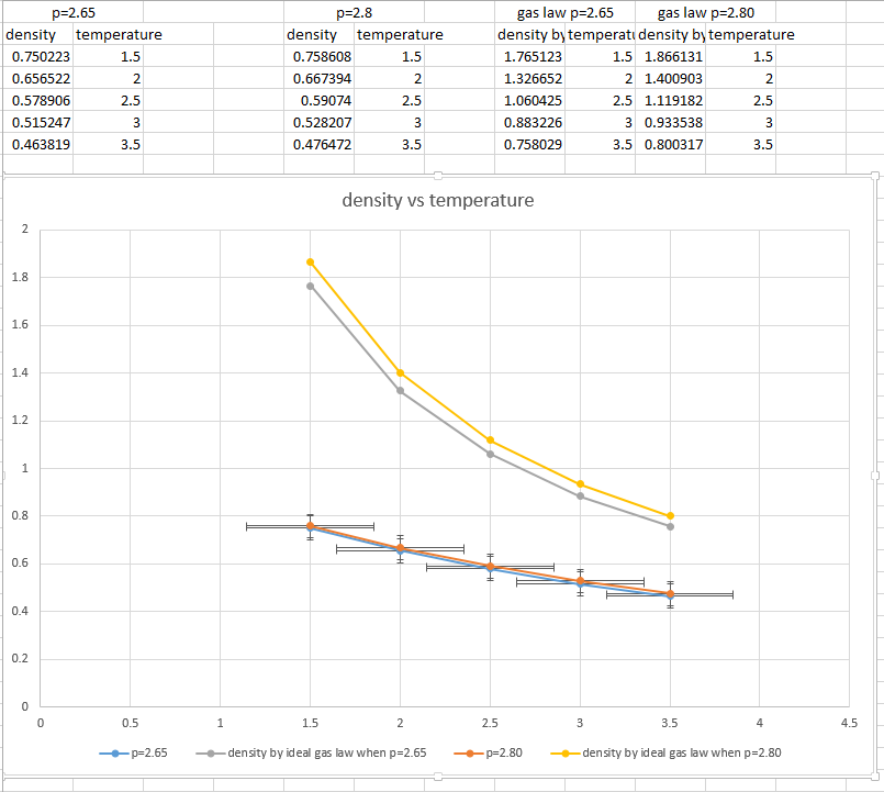
• plot of density vs temperature with error bars. a line corresponding to the density predicted by the ideal law.

The plot is obtained.

The density predicted by the ideal law can be calculated with $PV=nRT$${\left(5\right)}^{}$, and $N/V$ is density so $p=density*RT$</math>${\left(5\right)}^{}$

Task

• Is your simulated density lower or higher? Does the discrepancy increase or decrease with pressure?

Corresponding to the graph above, the simulated density is lower than the density calculated by ideal gas law.

As the gas law assumes no intermolecular forces between the gas molecules. This means molecules in gas phases can stick together without considering the intermoleclar forces, which indicates that the density calculated by ideal gas law should be higher than the real density. ${\left(5\right)}^{}$

According to the graph above, the discrepancy increases with pressure.

JC: The lack of intermolecular forces does allow the ideal gas to have a higher density than in the simulation, but how can molecules stick together without intermolecular forces?

Heat Capacity

Task

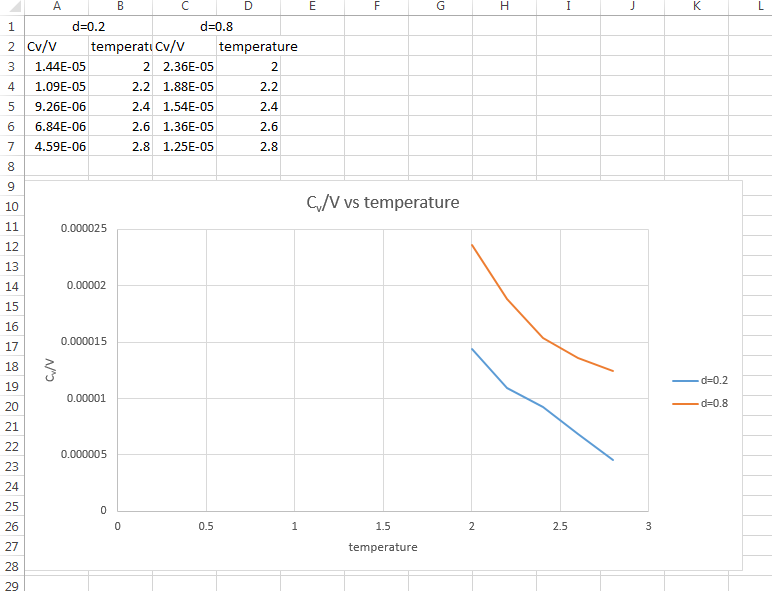
• Plot C_V/V as a function of temperature. Attach an input script.

The plot of Cv/V vs Temperature is obtained.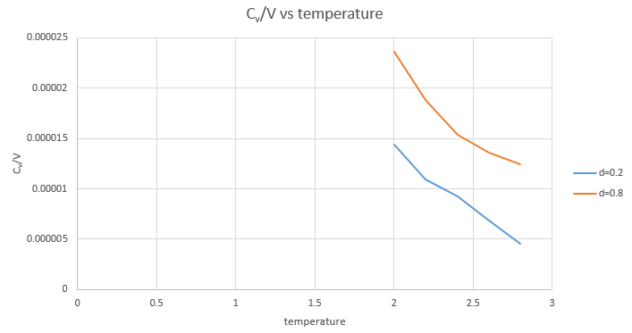

• Is the trend the one you would expect?

Yes. As shown in the graph, Cv/V decreases with the increasing temperature. (V remain the same when the density remain the same) As $C_V=\frac{\partial E}{\partial T}$${\left(1\right)}^{}$, the graph is consistent with the theory.

JC: Don't connect the data points in the graph with straight lines as it suggests that the heat capacity follows this trend between points. The definition of the heat capacity as dE/dT does not explain why heat capacity should increase or decrease with temperature.

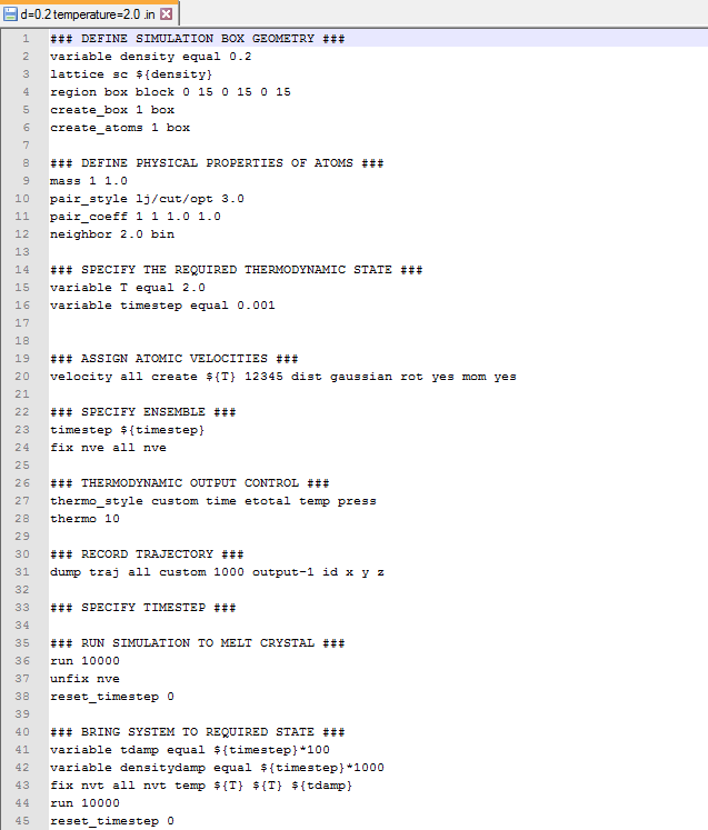
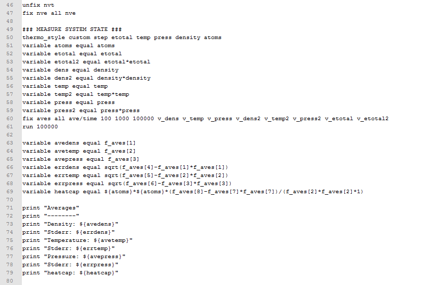
• An input scripts when density=0.2 and temperature=2.0 (see below)

Radical distribution Function

Task

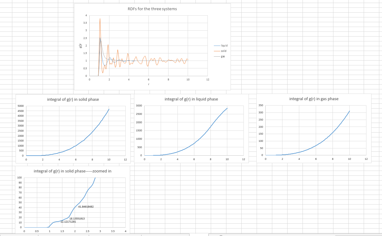
• calculate $g(r)$ and $\int g(r)\mathrm{d}r$. Plot the RDFs for the three systems on the same axes.

The plot of RDFs for three systems is obtained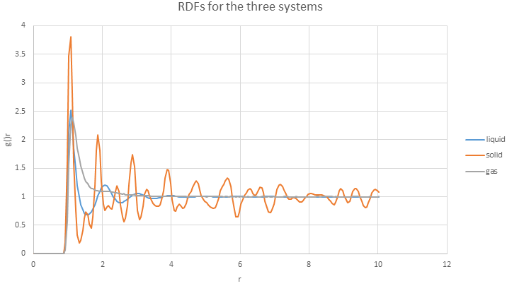

The RDF here is a function of the interatomic separation. Three RDFs all showing that at small r, the RDF is zero because of the atoms cannot approach any more closely due to the repulsion. Also, significant peaks indicate that atoms packed close to each other. Finally, as r increases, RDFs tend to be 1 because RDF is the average density at this range.${\left(6\right)}^{}$

• Qualitatively the differences between the three RDFs:

In solid, the atoms are at fixed lattice point, therefore, the peaks are very sharp.${\left(6\right)}^{}$ As the distance between atoms become further, the liquid is behaving like the gas, as there is no peaks.${\left(6\right)}^{}$

• The structure of the system in each phase.

In solid phase, the molecules are tightly bound to each other; in liquid phase, the molecules are more loosely bounded to each other which allows them to move; in gas phase, the molecules are free to move within a large distance.${\left(6\right)}^{}$

• In the solid case, illustrate which lattice sites the first three peaks correspond to. What is the lattice spacing? What is the coordination number for each of the first three peaks?

Integral of g(r) obtained

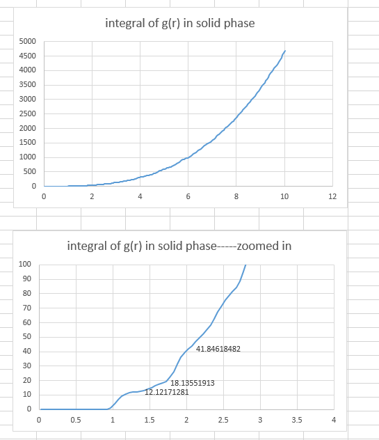
Three plateaus in integral of g(r) graph indicated the number of atoms that can be found at certain distances.

The first three peaks are the three shortest distances, which are 1.325, 1.675 and 2.025, between two lattice point in a fcc unit. The picture below illustrated these three distance.

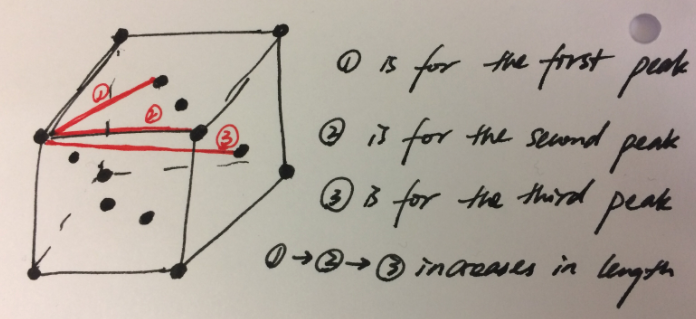
The lattice spacing is 1.675 indicated by the second data point (1.325, 0.187694215) on the solid RDF graph.

JC: Add a bit more detail to your explanation of the RDFs, the solid RDF shows long range order as the atoms are positioned on a lattice. The liquid RDF shows short range order, but no long range order. Good idea to include a diagram to show the atoms responsible for the first 3 peaks. Could you have calculated the lattice spacing from the first and third peaks as well and checked that it agreed with the value you have given?

Dynamic

Task

• a plot showing the "total" MSD vs timestep. Are these as you would expect? Estimate D in each case. Be careful with the units! Repeat this procedure for the MSD data that you were given from the one million atom simulations.

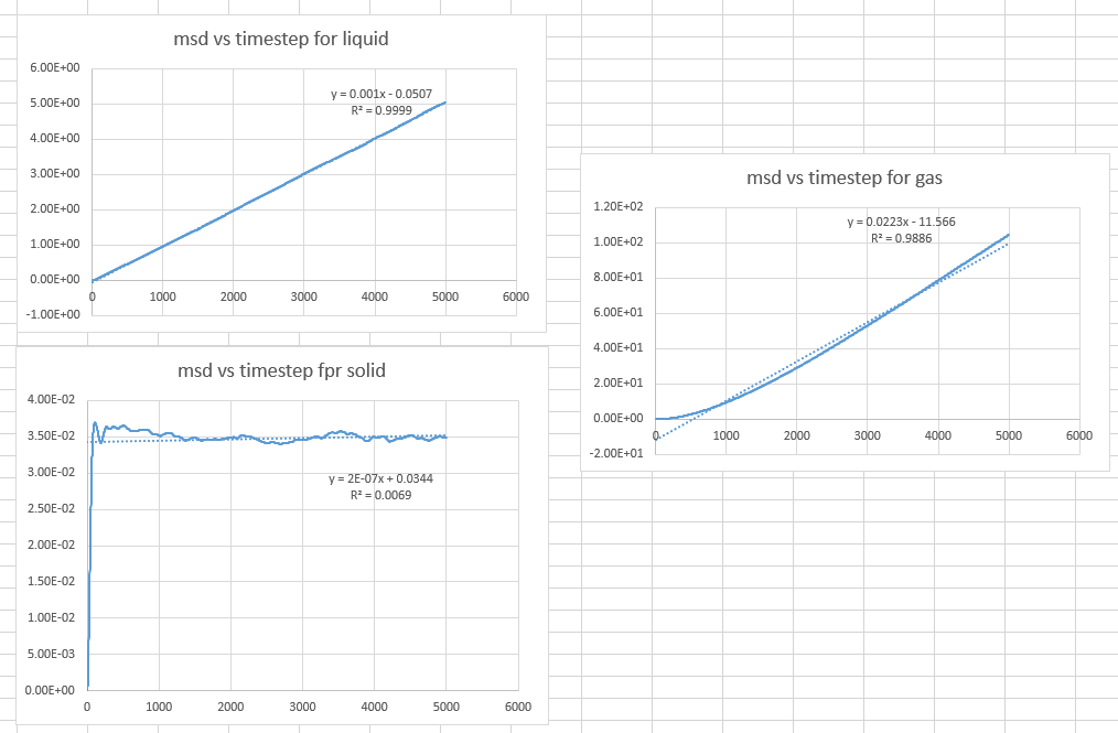
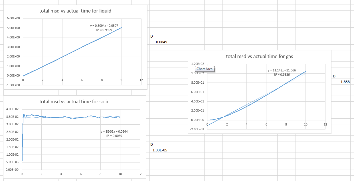
The plot is not linear for a short time in the gas graph. This is because the path a molecule takes will only be an approximate straight line until it collides with its neighbour. In gas, the molecule ate far away from each other, therefore this is what we would expect.

• Estimate D in each case

As $D=\frac{1}{6}\frac{\partial ⟨r^2\left(t\right)⟩}{\partial t}$${\left(7\right)}^{}$, to find $D$ is to plot a graph of total MSD vs actual time.

Then we get the slope from the graph which is $\frac{\partial ⟨r^2\left(t\right)⟩}{\partial t}$

Therefore we can calculate $D$. (the values are in the picture below) The solid phase does not have a diffusion coefficient because the atoms are not diffusing.

• the same procedure with the one million atom simulations

Again, The solid phase does not have a diffusion coefficient because the atoms are not diffusing.

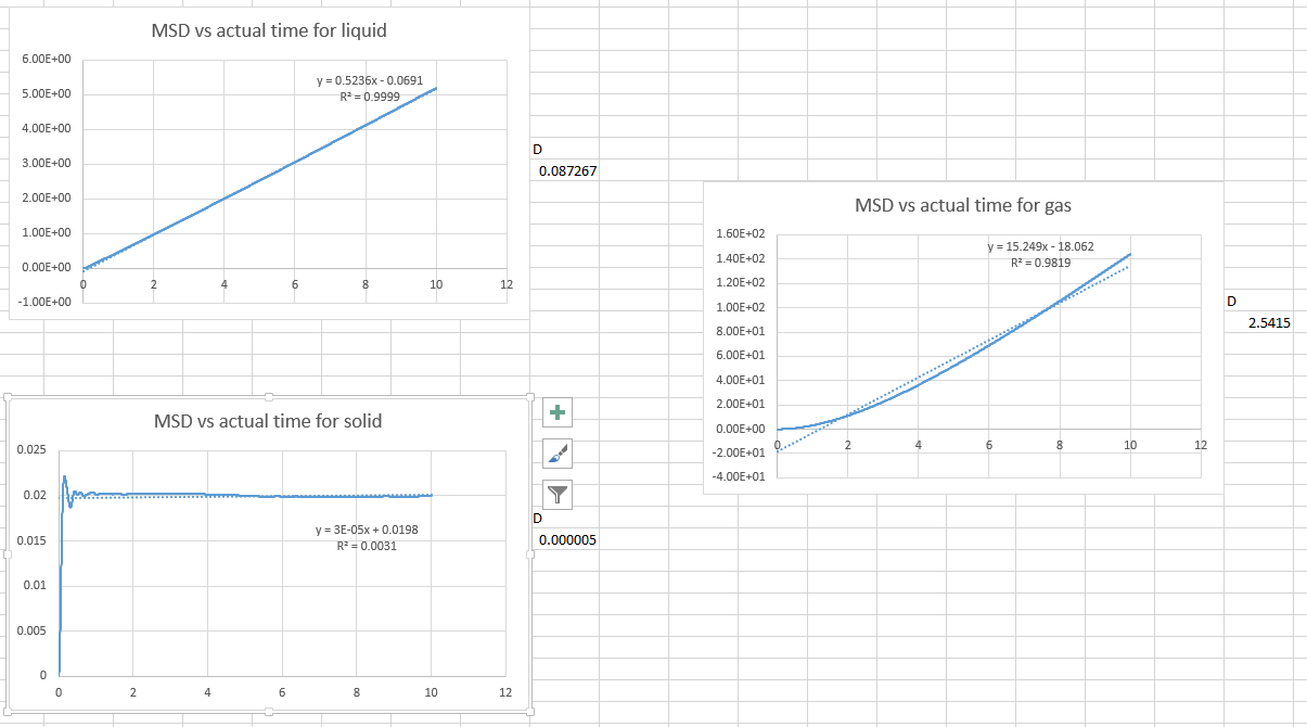
JC: The equation relating the mean squared displacement to the diffusion coefficient is only valid when mean squared displacement is linear so you should only fit this part of the graph.

Task

• evaluate C(τ) , plot C(τ) vs timestep and VACF vs timestep

The answer is $C\left(\tau \right)=cos\left(\omega \tau \right)$

The procedure of the evaluation is below

The position of a 1D harmonic oscillator as a function of time is $x\left(t\right)=A\cos (\omega t+\varphi )$${\left(1\right)}^{}$

$V\left(t\right)=\frac{\mathrm{d}x\left(t\right)}{\mathrm{d}t}$${\left(1\right)}^{}$

Thus $V\left(t\right)=-A\omega sin(\omega t+\varphi )$

As given $C\left(\tau \right)=\frac{\underset{-\mathrm{\infty }}{\overset{\mathrm{\infty }}{\int }}v\left(t\right)v(t+\tau )\mathrm{d}t}{\underset{-\mathrm{\infty }}{\overset{\mathrm{\infty }}{\int }}{v}^2\left(t\right)\mathrm{d}t}$

Thus $C\left(\tau \right)=\frac{\underset{-\mathrm{\infty }}{\overset{\mathrm{\infty }}{\int }}sin(\omega t+\varphi )sin(\omega t+\omega \tau +\varphi )dt}{\underset{-\mathrm{\infty }}{\overset{\mathrm{\infty }}{\int }}si{n}^2(\omega t+\varphi )dt}$

Fist, we work on the denominator which is $\underset{-\mathrm{\infty }}{\overset{\mathrm{\infty }}{\int }}si{n}^2(\omega t+\varphi )dt$

As we know $si{n}^2(\omega t+\varphi )=\frac{1}{2}-\frac{1}{2}cos(2\omega t+2\varphi )$

Thus $\underset{-\mathrm{\infty }}{\overset{\mathrm{\infty }}{\int }}si{n}^2(\omega t+\varphi )dt=\underset{-\mathrm{\infty }}{\overset{\mathrm{\infty }}{\int }}\frac{1}{2}dt-\underset{-\mathrm{\infty }}{\overset{\mathrm{\infty }}{\int }}\frac{1}{2}cos(2\omega t+2\varphi )dt$

Therefore, $\underset{-\mathrm{\infty }}{\overset{\mathrm{\infty }}{\int }}si{n}^2(\omega t+\varphi )dt={[\frac{1}{2}t-\frac{1}{4}\omega \times sin(2\omega t+2\varphi )]}_{-\mathrm{\infty }}^{\mathrm{\infty }}$

Secondly, we work on the numerator which is $\underset{-\mathrm{\infty }}{\overset{\mathrm{\infty }}{\int }}sin(\omega t+\varphi )sin(\omega t+\omega \tau +\varphi )dt$

Expand the sin equation, $\underset{-\mathrm{\infty }}{\overset{\mathrm{\infty }}{\int }}sin(\omega t+\varphi )sin(\omega t+\omega \tau +\varphi )dt=\underset{-\mathrm{\infty }}{\overset{\mathrm{\infty }}{\int }}sin(\omega t+\varphi )(sin(\omega t+\varphi )cos\left(\omega \tau \right)+cos(\omega t+\tau )sin\left(\omega \tau \right)))dt$

As $cos\left(\omega \tau \right)$ and $sin\left(\omega \tau \right)$ are constant

$\underset{-\mathrm{\infty }}{\overset{\mathrm{\infty }}{\int }}sin(\omega t+\varphi )sin(\omega t+\omega \tau +\varphi )dt=cos\left(\omega \tau \right)\underset{-\mathrm{\infty }}{\overset{\mathrm{\infty }}{\int }}si{n}^2(\omega t+\varphi )dt+sin\left(\omega \tau \right)\underset{-\mathrm{\infty }}{\overset{\mathrm{\infty }}{\int }}sin(\omega t+\varphi )cos(\omega t+\varphi )dt$

We already know $\underset{-\mathrm{\infty }}{\overset{\mathrm{\infty }}{\int }}si{n}^2(\omega t+\varphi )dt={[\frac{1}{2}t-\frac{1}{4}\omega \times sin(2\omega t+2\varphi )]}_{-\mathrm{\infty }}^{\mathrm{\infty }}$

Therefore, we are focusing on $sin\left(\omega \tau \right)\underset{-\mathrm{\infty }}{\overset{\mathrm{\infty }}{\int }}sin(\omega t+\varphi )cos(\omega t+\varphi )dt$this part

Let $U=sin(\omega t+\varphi )$

Thus $\frac{\mathrm{d}U}{\mathrm{d}t}=\frac{1}{\omega }cos(\omega t+\varphi )$

Substitute $cos(\omega t+\varphi )$ back in $sin\left(\omega \tau \right)\underset{-\mathrm{\infty }}{\overset{\mathrm{\infty }}{\int }}sin(\omega t+\varphi )cos(\omega t+\varphi )dt$

Therefore we get $sin\left(\omega \tau \right)\underset{-\mathrm{\infty }}{\overset{\mathrm{\infty }}{\int }}U\omega dU$

Thus $sin\left(\omega \tau \right)\underset{-\mathrm{\infty }}{\overset{\mathrm{\infty }}{\int }}sin(\omega t+\varphi )cos(\omega t+\varphi )dt={\left[\frac{1}{2}\omega sin\left(\omega \tau \right)si{n}^2(\omega t+\varphi )\right]}_{-\mathrm{\infty }}^{\mathrm{\infty }}$

Therefore, $C\left(\tau \right)=\frac{{[cos\left(\omega \tau \right)\times \frac{1}{2}t-\frac{1}{4}\omega cos\left(\omega \tau \right)sin(2\omega t+2\varphi )+\frac{1}{2}\omega sin\left(\omega \tau \right)si{n}^2(\omega t+\varphi )]}_{-\mathrm{\infty }}^{\mathrm{\infty }}}{{[\frac{1}{2}t-\frac{1}{4}sin(2\omega t+2\varphi )]}_{-\mathrm{\infty }}^{\mathrm{\infty }}}$

As t tends to infinity, $C\left(\tau \right)=\frac{cos\left(\omega \tau \right)\times \frac{1}{2}t}{\frac{1}{2}t}$

Thus $C\left(\tau \right)=cos\left(\omega \tau \right)$

JC: You don't need to do all of the integration, you should be able to simplify the expression first.

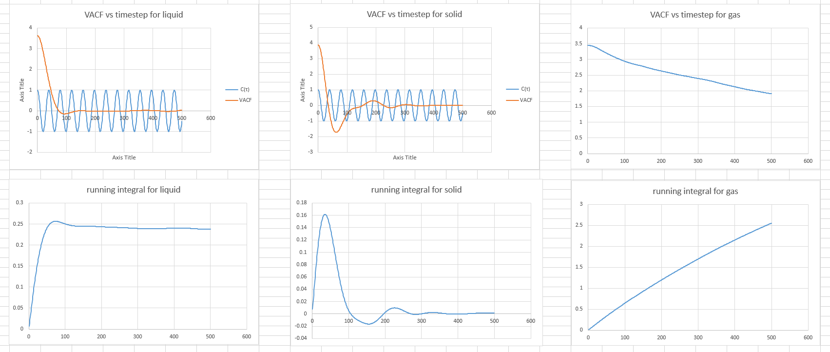
Plot obtained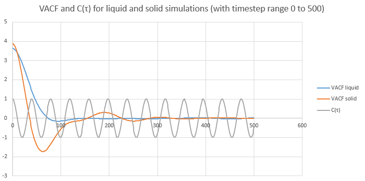 The minima in the VACFs for the liquid and solid system represent very damped oscillations. The oscillation is a collision between two atoms.${\left(9\right)}^{}$

Even though liquid behave similarly to solids, atoms are stil close to each other, there are differences between the liquid and solid VACFs. ${\left(9\right)}^{}$

Because in solid the atoms are a fixed positions, their motion is an oscillation. This is why we have a function that oscillates strongly from positive to negative value and back again.${\left(9\right)}^{}$

In liquid, two atoms collide before they diffuse away.${\left(9\right)}^{}$

The harmonic oscillator VACF is cos(ωτ) vs time. Since $\omega =1/2\pi$, τ the timestep is the variable here. Since cos function is a periodic function, the shape of harmonic oscillator VACF is very different to the Lennard Jones solid and liquid.

JC: Why do the solid and liquid VACFs decay to zero, but the harmonic oscillator does not?

Task

• Use the trapezium rule to approximate the integral under the velocity autocorrelation function for the solid, liquid, and gas, and use these values to estimate D in each case. Are they as you expect? What do you think is the largest source of error in your estimates of D from the VACF?

With $\underset{a}{\overset{b}{\int }}f(x)dx\approx \frac{h}{2}\sum _{k=1}^N(f(x_{k+1})+f(x_k))$ ${\displaystyle }=\frac{b-a}{2N}(f(x_1)+2f(x_2)+2f(x_3)+2f(x_4)+\cdots +2f(x_N)+f(x_{N+1})).$ ${\left(12\right)}^{}$equation, the integral under VACF is 0.803506332 in solid, 119.1372588 in liquid and 1277.155395 in gas.

Therefore, the D in solid phase is 0.267835444, in liquid phase is 39.71241959 and in gas phase is 425.718465.

As $D=\frac{1}{3}\underset{0}{\overset{\mathrm{\infty }}{\int }}\mathrm{d}\tau ⟨\mathbf{v}\left(0\right)\cdot \mathbf{v}\left(\tau \right)⟩$${\left(1\right)}^{}$, we can calculate D by dividing the integral under the velocity autocorrelation function by three.

• A plot of the running integral

According to the graphs of VACF vs timestep, the running integral plots are reasonable.

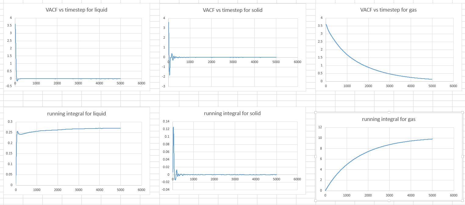
• Repeat this procedure for the VACF data that you were given from the one million atom simulations.

With same approach as before, the integral under VACF is 0.068294227 in solid, 135.1372144 in liquid and 4902.698697in gas.

Therefore, the D in solid phase is 0.022764742, in liquid phase is 45.04573814 and in gas phase is 1634.232899.

Conclusion&Summary

• We run the simulations with different timesteps to compare which timestep is more accurate.
• With the velocity-Verlet algorithm and the Lennard-Jones potential, boundary conditions and reduce unit, we understand the theory for the simulation.
• Analyse the output of the simulation with thermodynamic properties to check the equilibrium.
• Under NpT conditions, plotting the equation of different states.
• Heat capacities are obtained in density-temperature phase space with the calculation of statistical physics.
• Radical distribution functions are obtained to understand how, on average, the atoms in a system are radially packed around each other.
• Mean Squared Displacement and Velocity Autocorrelation Function are obtained to understand how the square distance grows with time (since is squared, it will not be sums up to zero with both positive and negative values )

References

${\left(1\right)}^{}$ Chemistry Wiki, https://wiki.ch.ic.ac.uk/wiki/index.php?title=Third_year_simulation_experiment, (accessed October 2016).

${\left(2\right)}^{}$ Chemistry libretexts, http://chem.libretexts.org/Core/Physical_and_Theoretical_Chemistry/Physical_Properties_of_Matter/Atomic_and_Molecular_Properties/Intermolecular_Forces/Specific_Interactions/Lennard-Jones_Potential, (accessed October 2016).

${\left(3\right)}^{}$ The physics classroom, http://www.physicsclassroom.com/calcpad/energy, (accessed October 2016).

${\left(4\right)}^{}$ Lammps, http://lammps.sandia.gov/doc/Section_commands.html#cmd_5, (accessed October 2016).

${\left(5\right)}^{}$ University of Oregan, http://abyss.uoregon.edu/~js/glossary/ideal_gas_law.html, (accessed October 2016).

${\left(6\right)}^{}$ Democritus, http://www.ccp5.ac.uk/DL_POLY/Democritus/Theory/rdf.html, (accessed November 2016).

${\left(7\right)}^{}$ Democritus, http://www.ccp5.ac.uk/DL_POLY/Democritus/Theory/msd.html, (accessed November 2016).

${\left(8\right)}^{}$ Democritus, http://www.ccp5.ac.uk/DL_POLY/Democritus/Theory/msd2.html, (accessed November 2016).

${\left(9\right)}^{}$ Democritus, http://www.ccp5.ac.uk/DL_POLY/Democritus/Theory/vaf.html, (accessed November 2016).

${\left(10\right)}^{}$ Faculty of Physcis, http://phys.ubbcluj.ro/~tbeu/MD/C2_for.pdf, (accessed November 2016).

${\left(11\right)}^{}$ Jean-Pierre Hansen and Loup Verlet, Phys. Rev., 1969, 184, 151

${\left(12\right)}^{}$ Revision Maths, https://revisionmaths.com/advanced-level-maths-revision/pure-maths/calculus/trapezium-rule, (accessed November 2016).

Appendix

Some other graphs with data obtained