Talk:NBCMP

Introduction to the Ising Model

TASK: Show that the lowest possible energy for the Ising model is $E = - D N J$ , where $D$ is the number of dimensions and $N$ is the total number of spins. What is the multiplicity of this state? Calculate its entropy.

If a spin of +1 is assigned to each cell this would be the lowest energy configuration as the spins are parallel. Using $- \frac{1}{2} J \sum_{i}^{N} \sum_{j \in n e i g h b o u r s (i)} s_{i} s_{j}$ . Taking the example of a 1D model, counting the interaction of each adjacent cell in one direction (including the periodic boundary condition that the final spin is adjacent to the first) and multiplying this by 2 to include interactions in the opposite direction, the factor of ½ cancels out due to the inclusion of interactions in both directions. Therefore the energy for this model would be -5 – where D=1 and N=5, as the model is 1 dimension with 5 spins.

Using a 2D model of 5x5 and the same system, the total number of interactions is 50, when each column and row is considered. This again corresponds to the $E = - D N J$ where D=2 and N=25.

NJ: better to argue as follows: in $D$ dimensions, every spin has $2 D$ neighbours. Every spin therefore contributes $- 2 D J$ to the energy when all spins are aligned (up or down). Doing the sum, then applying the factor of 0.5, gives $E = - D N J$ .

The entropy would be equal to S=k_b ln W, where k_b is the Boltzmann constant and W the number of microstates in a system. We take W=2 in this case as the multiplicity (spins of -1 or +1) is 2. Therefore S = 1.38 x 10^-23 x ln(2) = 9.565 x 10^-24 JK^-1

NJ: good.

TASK: Imagine that the system is in the lowest energy configuration. To move to a different state, one of the spins must spontaneously change direction ("flip"). What is the change in energy if this happens (D=3,\ N=1000)? How much entropy does the system gain by doing so?

The energy of this system using the EQUATION is -3000J, where all spins are parallel and +1. Being in 3D system, one spin has interactions with 6 other spins. On the changing of one spin, i.e. from +1 to -1, this causes the removal of 6 previously favourable interactions and the gain of 6 unfavourable interactions, resulting in a change in energy of 12J.

NJ: correct

Using the equation S = k_b lnW where W = N!/SUM n!, W = 1000! x 2/999!, as there are 1000 spins, with a multiplicity of 2, but one spin is defined as the opposite, accounting for the denominator 999!. This gives a result of S = 1.38 x 10^-23 x ln(2000) = 1.049 x 10^-22 ^-1.

NJ: this is correct, but the question asks how much entropy is gained. $Δ S = k_{B} \ln (\frac{2 N}{2}) = k_{B} \ln 1000$

TASK: Calculate the magnetisation of the 1D and 2D lattices in figure 1. What magnetisation would you expect to observe for an Ising lattice with $D = 3$ $N = 1000$ at absolute zero?

Magnetisation of the 1D lattice is +3 – 2 = +1. Magnetisation of the 2D lattice is +13 – 12 = +1.

At absolute zero the lattice would take the lowest energy configuration with all spins parallel, i.e. all spins either +1 or all spins -1. Therefore the magnetisation would be either +1000 or -1000.

NJ: good!

Calculating the energy and magnetisation

TASK: complete the functions energy() and magnetisation(), which should return the energy of the lattice and the total magnetisation, respectively. In the energy() function you may assume that at all times (in fact, we are working in reduced units in which , but there will be more information about this in later sections). Do not worry about the efficiency of the code at the moment — we will address the speed in a later part of the experiment.

Python Code

import numpy as np

class IsingLattice:

    E = 0.0
    E2 = 0.0
    M = 0.0
    M2 = 0.0

    n_cycles = 0

    def __init__(self, n_rows, n_cols):
        self.n_rows = n_rows
        self.n_cols = n_cols
        self.lattice = np.random.choice([-1,1], size=(n_rows, n_cols))

    def energy(self):
        "Return the total energy of the current lattice configuration."
        #creates an empty list for the energy
        energy = []
        #when the element is at the end of the column or row, this uses the periodic boundary condition
        for i in range(self.n_rows):
                for k in range(self.n_cols):
                    if k<(self.n_cols-1):
                        energy.append(self.lattice[i,k]*self.lattice[i,k+1]*2)
                    else:
                        energy.append(self.lattice[i,k]*self.lattice[i,0]*2)
                    if i<(self.n_cols-1):
                        energy.append(self.lattice[i,k]*self.lattice[i+1,k]*2)
                    else:
                        energy.append(self.lattice[i,k]*self.lattice[0,k]*2)
                        
        energy = -0.5*sum(energy)

        return energy

    def magnetisation(self):
        "Return the total magnetisation of the current lattice configuration."
        #magnetisation is the sum of spins
        magnetisation = np.sum(self.lattice)
        return magnetisation

NJ: a little more explanation of the energy() function would be good. The following are pointers for general good practice (you weren't penalised for them because this section isn't about performance):

storing all of the energy contributions in a list is a bad idea — you are using memory needlessly, you could just keep a running total of the energy
you don't need to multiply the interactions by 2, then divide by 2 at the end. You can just single count in the loop.

TASK: Run the ILcheck.py script from the IPython Qt console using the command The displayed window has a series of control buttons in the bottom left, one of which will allow you to export the figure as a PNG image. Save an image of the ILcheck.py output, and include it in your report.

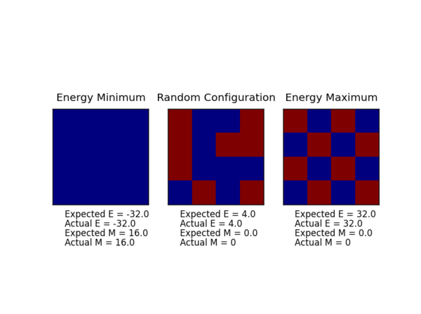
NJ: nice!

Introduction to Monte Carlo Simulation

TASK: How many configurations are available to a system with 100 spins? To evaluate these expressions, we have to calculate the energy and magnetisation for each of these configurations, then perform the sum. Let's be very, very, generous, and say that we can analyse $1 \times 1 0^{9}$ configurations per second with our computer. How long will it take to evaluate a single value of ${⟨ M ⟩}_{T}$ ?

For a system with 100 spins there are 2¹⁰⁰ spins available. This means it would take 1.267 x 10²¹ seconds to evaluate a single value of ${⟨ M ⟩}_{T}$ .

NJ: how long is this in "real time"?

TASK: Implement a single cycle of the above algorithm in the montecarlocycle(T) function. This function should return the energy of your lattice and the magnetisation at the end of the cycle. You may assume that the energy returned by your energy() function is in units of $k_{B}$ ! Complete the statistics() function. This should return the following quantities whenever it is called: $< E >, < E^{2} >, < M >, < M^{2} >$ , and the number of Monte Carlo steps that have elapsed.

def montecarlostep(self, T):
        # complete this function so that it performs a single Monte Carlo step
        #the following two lines will select the coordinates of the random spin for you
        #self.lattice = np.random.choice([-1,1], size=(self.n_rows, self.n_cols))
        random_i = np.random.choice(range(1, self.n_rows))
        random_j = np.random.choice(range(1, self.n_cols))

        #energy of original lattice
        energy = []
        for i in range(self.n_rows):
            for k in range(self.n_cols):
                if k<(self.n_cols-1):
                    energy.append(self.lattice[i,k]*self.lattice[i,k+1]*2)
                else:
                    energy.append(self.lattice[i,k]*self.lattice[i,0]*2)
                if i<(self.n_cols-1):
                    energy.append(self.lattice[i,k]*self.lattice[i+1,k]*2)
                else:
                    energy.append(self.lattice[i,k]*self.lattice[0,k]*2)
                        
        energy = -0.5*sum(energy)

        #selects random coordinates and flips spin for new lattice
        self.lattice[random_i,random_j]=self.lattice[random_i,random_j]*-1     

        #energy of new lattice
        energyb = []
        for i in range(self.n_rows):
            for k in range(self.n_cols):
                if k<(self.n_cols-1):
                    energyb.append(self.lattice[i,k]*self.lattice[i,k+1]*2)
                else:
                    energyb.append(self.lattice[i,k]*self.lattice[i,0]*2)
                if i<(self.n_cols-1):
                    energyb.append(self.lattice[i,k]*self.lattice[i+1,k]*2)
                else:
                    energyb.append(self.lattice[i,k]*self.lattice[0,k]*2)
        
        
        energyb = -0.5*sum(energyb)
        #change in energy calculated by
        energydiff = energyb - energy

        #uses criteria to return energy of the lowest energy configuration      
        if energydiff<0:
            self.lattice=self.lattice
        #the following line will choose a random number in the rang e[0,1) for you
        else:
            random_number = np.random.random()
            if random_number<= np.exp(-energydiff/(T)):
                self.lattice=self.lattice
                energy=energyb
            else:
                self.lattice[random_i,random_j]=self.lattice[random_i,random_j]*-1
                energy=energy
                
                
        #calculates both the energy and magnetisation
        #ignores 500 cycles when calculating the average statistics in the next step
        magnetisation = np.sum(self.lattice)
        self.n_cycles=self.n_cycles+1
        
        if self.n_cycles>500:
            self.E += energy
            self.M += magnetisation
            self.E2 += energy*energy
            self.M2 += magnetisation*magnetisation
        return energy, magnetisation

               #returns the statistic values for future calculations 
    def statistics(self):
        
        aveE = self.E/(self.n_cycles-500)
        aveE2 = (self.E2)/(self.n_cycles-500)
        aveM = self.M/(self.n_cycles-500)
        aveM2 = (self.M2)/(self.n_cycles-500)
        n_cycles = (self.n_cycles-500)
        
        return aveE, aveE2, aveM, aveM2, n_cycles

NJ: I think this might be an older version of your code - the MC steps only select random numbers in the range [1,N), instead of [0,N). I think we talked about this at some stage, and your simulation looks good in any case. You should also be suing the energy() function instead of calculating the energy each time you need it.

TASK: If $T < T_{C}$ , do you expect a spontaneous magnetisation (i.e. do you expect $⟨ M ⟩ \neq 0$ )? When the state of the simulation appears to stop changing (when you have reached an equilibrium state), use the controls to export the output to PNG and attach this to your report. You should also include the output from your statistics() function.


Simulation image	Statistics data
	Averaged quantities: E = -1.95763888889 EE = 3.83747829861 M = 0.987413194444 MM = 0.975485568576 number of cycles = 360

NJ: Do you expect spontaneous magnetisation when $T < T_{C}$ ?

Accelerating the code

TASK: Use the script ILtimetrial.py to record how long your current version of IsingLattice.py takes to perform 2000 Monte Carlo steps. This will vary, depending on what else the computer happens to be doing, so perform repeats and report the error in your average!


Original code run time	Data analysis
Time (s) 3.27015288 3.235212669 3.280651545 3.244010659 3.248185675 3.23469649 3.237294894 3.277660723 3.254181204 3.233904109	Average/mean = 3.251595085 Standard error = ±1.02760869

TASK: Look at the documentation for the NumPy sum function. You should be able to modify your magnetisation() function so that it uses this to evaluate M. The energy is a little trickier. Familiarise yourself with the NumPy roll and multiply functions, and use these to replace your energy double loop (you will need to call roll and multiply twice!).

Originally the magnetisation was calculated using the NumPy function.

class IsingLattice:

    E = 0.0
    E2 = 0.0
    M = 0.0
    M2 = 0.0

    n_cycles = 0

    def __init__(self, n_rows, n_cols):
        self.n_rows = n_rows
        self.n_cols = n_cols
        self.lattice = np.random.choice([-1,1], size=(n_rows, n_cols))

    def energy(self):
        "Return the total energy of the current lattice configuration."
        interaction1 = np.multiply(np.roll(self.lattice, 0, axis=1), np.roll(self.lattice, 1, axis=1))
        interaction2 = np.multiply(np.roll(self.lattice, 0, axis=0), np.roll(self.lattice, 1, axis=0))
        totalsum = np.sum([interaction1, interaction2])
        energy = -1*totalsum
        return energy

    def magnetisation(self):
        "Return the total magnetisation of the current lattice configuration."
        magnetisation = np.sum(self.lattice)
        return magnetisation

NJ: You don't need to do roll with an offset of 0, you can just use the self.lattice variable. I would also avoid making the list, and just do something like:

 energy = 0

 energy -= np.sum(np.multiply(self.lattice, np.roll(self.lattice, 1, axis=0)))

 energy -= np.sum(np.multiply(self.lattice, np.roll(self.lattice, 1, axis=1)))

TASK: Use the script ILtimetrial.py to record how long your new version of IsingLattice.py takes to perform 2000 Monte Carlo steps. This will vary, depending on what else the computer happens to be doing, so perform repeats and report the error in your average!


Original code run time	Data analysis
Time (s) 0.180072049 0.183888848 0.180241095 0.189717888 0.18089373 0.181124959 0.181679488 0.186710997 0.180462363 0.1811962	Average/mean = 0.182598762 Standard error = ±0.057840506

The effect of temperature

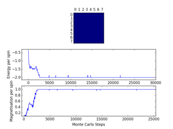
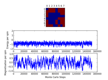
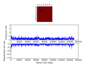
TASK: The script ILfinalframe.py runs for a given number of cycles at a given temperature, then plots a depiction of the final lattice state as well as graphs of the energy and magnetisation as a function of cycle number. This is much quicker than animating every frame! Experiment with different temperature and lattice sizes. How many cycles are typically needed for the system to go from its random starting position to the equilibrium state? Modify your statistics() and montecarlostep() functions so that the first N cycles of the simulation are ignored when calculating the averages. You should state in your report what period you chose to ignore, and include graphs from ILfinalframe.py to illustrate your motivation in choosing this figure.

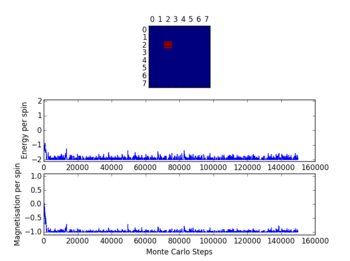
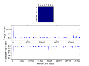
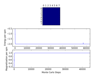
Looking at the diagram for a temperature of 1.2, the time to reach the equilibrium state is quite low, so 500 cycles are being discounted in calculating the averages. For higher temperatures i.e. 2 and 3, the fluctuations are rapid and cannot be used to pass judgement. At higher temperatures the entropic contribution dominates (as opposed to energetic) and the equilibrium state takes longer to reach - this can be seen from the diagrams.

NJ: It's quite hard to see from your graphs if 500 cycles is enough. How does the lattice size affect this?

	Temperature
1.0	3.0	2.0	1.5	1.2	0.8

TASK: Use ILtemperaturerange.py to plot the average energy and magnetisation for each temperature, with error bars, for an $8 \times 8$ lattice. Use your initution and results from the script ILfinalframe.py to estimate how many cycles each simulation should be. The temperature range 0.25 to 5.0 is sufficient. Use as many temperature points as you feel necessary to illustrate the trend, but do not use a temperature spacing larger than 0.5. T NumPy function savetxt() stores your array of output data on disk — you will need it later. Save the file as 8x8.dat so that you know which lattice size it came from.

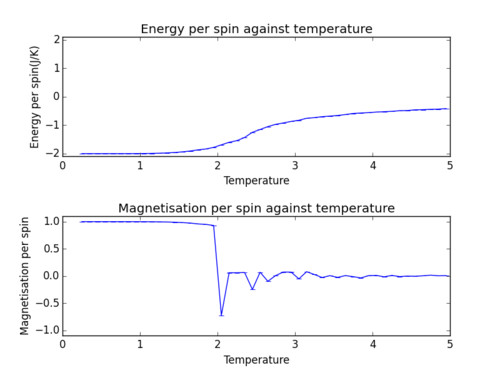
NJ: How many Monte Carlo steps did you perform for each temperature?

The effect of system size

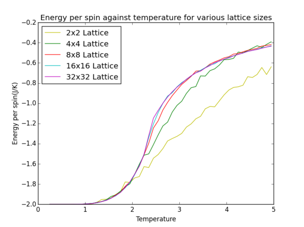
TASK: Repeat the final task of the previous section for the following lattice sizes: 2x2, 4x4, 8x8, 16x16, 32x32. Make sure that you name each datafile that your produce after the corresponding lattice size! Write a Python script to make a plot showing the energy per spin versus temperature for each of your lattice sizes. Hint: the NumPy loadtxt function is the reverse of the savetxt function, and can be used to read your previously saved files into the script. Repeat this for the magnetisation. As before, use the plot controls to save your a PNG image of your plot and attach this to the report. How big a lattice do you think is big enough to capture the long range fluctuations?

from IsingLattice import *
from matplotlib import pylab as pl
import numpy as np

#load data from files
data2 = np.loadtxt("2x2(2).dat")
data4 = np.loadtxt("4x4(2).dat")
data8 = np.loadtxt("8x8(2).dat")
data16 = np.loadtxt("16x16(2).dat")
data32 = np.loadtxt("32x32(2).dat")

#name plots and use pylab to plot x and y
lattice2 = pl.plot(data2[:,0], data2[:,1]/4, 'y', label='2x2 Lattice')
lattice4 = pl.plot(data4[:,0], data4[:,1]/16, 'g', label='4x4 Lattice')
lattice8 = pl.plot(data8[:,0], data8[:,1]/64, 'r', label='8x8 Lattice')
lattice16 = pl.plot(data16[:,0], data16[:,1]/256,'c', label= '16x16 Lattice')
lattice32 = pl.plot(data32[:,0], data32[:,1]/1024, 'm', label= '32x32 Lattice')

#axis labels
pl.xlabel('Temperature')
pl.ylabel('Energy per spin(J/K)')
pl.title('Energy per spin against temperature for various lattice sizes')

#make legend
pl.legend(loc='best', numpoints=1)

#show plot
pl.show()

NJ: You don't need to import the IsingLattice module here

from IsingLattice import *
from matplotlib import pylab as pl
import numpy as np

#load data from files
data2 = np.loadtxt("2x2(2).dat")
data4 = np.loadtxt("4x4(2).dat")
data8 = np.loadtxt("8x8(2).dat")
data16 = np.loadtxt("16x16(2).dat")
data32 = np.loadtxt("32x32(2).dat")

#name plots and use pylab to plot x and y
lattice2 = pl.plot(data2[:,0], data2[:,3]/4, 'y', label='2x2 Lattice')
lattice4 = pl.plot(data4[:,0], data4[:,3]/16, 'g', label='4x4 Lattice')
lattice8 = pl.plot(data8[:,0], data8[:,3]/64, 'r', label='8x8 Lattice')
lattice16 = pl.plot(data16[:,0], data16[:,3]/256,'c', label= '16x16 Lattice')
lattice32 = pl.plot(data32[:,0], data32[:,3]/1024, 'm', label= '32x32 Lattice')

#axis labels
pl.xlabel('Temperature')
pl.ylabel('Magnetisation per spin')
pl.title('Magnetisation per spin against temperature for various lattice sizes')

#make legend
pl.legend(loc='best', numpoints=1)

#show plot
pl.show()

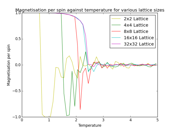
A lattice size of 8x8 is large enough to capture long range fluctuations as it yields similar results to a 32x32 lattice without having to invest in large calculation times.

Determining the heat capacity

TASK: Write a Python script to make a plot showing the heat capacity versus temperature for each of your lattice sizes from the previous section. You may need to do some research to recall the connection between the variance of a variable, $V a r [X]$ , the mean of its square $⟨ X^{2} ⟩$ , and its squared mean ${⟨ X ⟩}^{2}$ . You may find that the data around the peak is very noisy — this is normal, and is a result of being in the critical region. As before, use the plot controls to save your a PNG image of your plot and attach this to the report.

from IsingLattice import *
from matplotlib import pylab as pl
import numpy as np

#load data from files
data32 = np.loadtxt("32x32(2).dat")

pl.title('Heat Capacity against Temperature')
pl.ylabel("Heat Capacity")
pl.xlabel("Temperature(K)")
pl.ylim([0,2])
energy_variance= np.subtract((data32[:,2]), (np.multiply((data32[:,1]), (data32[:,1]))))
heatcapacity=(energy_variance/(1024*(np.multiply((data32[:,0]), (data32[:,0])))))
heatcap =pl.plot((data32[:,0]), np.array(heatcapacity))

pl.show()

final_data = np.column_stack((data32[:,0], heatcapacity))
np.savetxt("hc32x32.dat", final_data)

NJ: A few more comments would be nice - for example "divide C by N to make comparison between systems easier"

Script to plot all heat capacities on one graph:

from IsingLattice import *
from matplotlib import pylab as pl
import numpy as np

#load data from files
data2 = np.loadtxt("hc2x2.dat")
data4 = np.loadtxt("hc4x4.dat")
data8 = np.loadtxt("hc8x8.dat")
data16 = np.loadtxt("hc16x16.dat")
data32 = np.loadtxt("hc32x32.dat")

#name plots and use pylab to plot x and y
lattice2 = pl.plot(data2[:,0], data2[:,1], 'y', label='2x2 Lattice')
lattice4 = pl.plot(data4[:,0], data4[:,1], 'g', label='4x4 Lattice')
lattice8 = pl.plot(data8[:,0], data8[:,1], 'r', label='8x8 Lattice')
lattice16 = pl.plot(data16[:,0], data16[:,1],'c', label= '16x16 Lattice')
lattice32 = pl.plot(data32[:,0], data32[:,1], 'm', label= '32x32 Lattice')

#axis labels
pl.xlabel('Temperature')
pl.ylabel('Heat Capacity(J/K)')
pl.title('Heat Capacity against temperature for various lattice sizes')

#make legend
pl.legend(loc='best', numpoints=1)

#show plot
pl.show()

The maximum in the heat capacity is referred to as the Schottky anomaly.

Locating the Curie temperature

TASK: A C++ program has been used to run some much longer simulations than would be possible on the college computers in Python. You can view its source code here if you are interested. Each file contains six columns: $T, E, E^{2}, M, M^{2}, C$ (the final five quantities are per spin), and you can read them with the NumPy loadtxt function as before. For each lattice size, plot the C++ data against your data. For one lattice size, save a PNG of this comparison and add it to your report — add a legend to the graph to label which is which. To do this, you will need to pass the label="..." keyword to the plot function, then call the legend() function of the axis object (documentation here).

NJ: Where is the plot comparing the C++ and Python data?

File name for loading data was changed according to the lattice size each time. In this example the 8x8 lattice size was used.

from IsingLattice import *
from matplotlib import pylab as pl
import numpy as np

#load data from C++ file
data8 = np.loadtxt("8x8.dat")
lattice8= pl.plot(data8[:,0], data8[:,5], 'y', label='Data')

#assume data is now a 2D array containing two columns, T and C
T = data8[:,0] #get the temperatures
C = data8[:,5] #get the heat capacity

#first we fit the polynomial to the data
fit = np.polyfit(T, C, 15) #fit a polynomial

#now we generate interpolated values of the fitted polynomial over the range of our function
T_min = np.min(T)
T_max = np.max(T)
T_range = np.linspace(T_min, T_max, 1000) #generate 1000 evenly spaced points between T_min and T_max
fitted_C_values = np.polyval(fit, T_range) #use the fit object to generate the corresponding values of C
poly= pl.plot(T_range, fitted_C_values, 'b', label='Polynomial fit')

pl.xlabel=('Temperature')
pl.ylabel=('Heat Capacity')
pl.title=('Polynomial fitting for Heat Capacity')

#make legend
pl.legend(loc='best', numpoints=1)

pl.show()

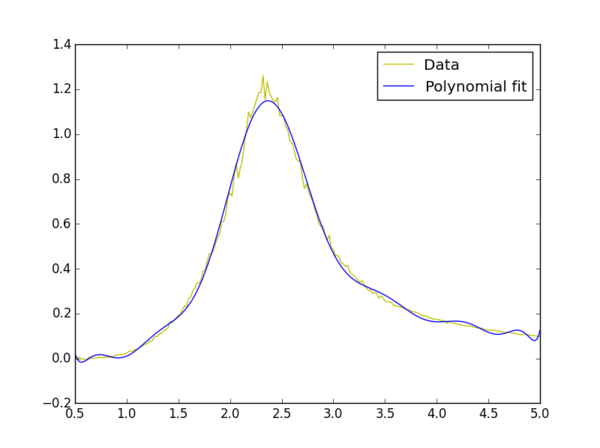
TASK: write a script to read the data from a particular file, and plot C vs T, as well as a fitted polynomial. Try changing the degree of the polynomial to improve the fit — in general, it might be difficult to get a good fit! Attach a PNG of an example fit to your report.

from IsingLattice import *
from matplotlib import pylab as pl
import numpy as np

#load data from file
data8 = np.loadtxt("8x8.dat")
lattice8= pl.plot(data8[:,0], data8[:,5], 'y', label='Data')

#assume data is now a 2D array containing two columns, T and C
T = data8[:,0] #get the first column
C = data8[:,5] # get the second column

#first we fit the polynomial to the data
fit = np.polyfit(T, C, 50) # fit a third order polynomial

#now we generate interpolated values of the fitted polynomial over the range of our function
Tmin = 1.5 
Tmax = 3.5 
selection = np.logical_and(T > Tmin, T < Tmax) #choose only those rows where both conditions are true
peak_T_values = T[selection]
peak_C_values = C[selection]
T_min = np.min(peak_T_values)
T_max = np.max(peak_T_values)
peak_T_range = np.linspace(T_min, T_max, 1000) #generate 1000 evenly spaced points between T_min and T_max
fitted_C_values = np.polyval(fit, peak_T_range) # use the fit object to generate the corresponding values of C
poly= pl.plot(peak_T_range, fitted_C_values, 'b', label='Polynomial fit')
pl.xlabel=('Temperature')
pl.ylabel=('Heat Capacity(J/K)')
pl.title=('Heat Capacity against Temperature with a polynomial fit') 

#make legend
pl.legend(loc='best', numpoints=1)

pl.show()

NJ: This fit isn't limited to the peak region! You generate the subset of temperatures correctly, but you still call polyfit on the whole range (you're not actually fitting to the subrange).

TASK: find the temperature at which the maximum in C occurs for each datafile that you were given. Make a text file containing two colums: the lattice side length (2,4,8, etc.), and the temperature at which C is a maximum. This is your estimate of $T_{C}$ for that side length. Make a plot that uses the scaling relation given above to determine $T_{C, \infty}$ . By doing a little research online, you should be able to find the theoretical exact Curie temperature for the infinite 2D Ising lattice. How does your value compare to this? Are you surprised by how good/bad the agreement is? Attach a PNG of this final graph to your report, and discuss briefly what you think the major sources of error are in your estimate.

NJ: How did you determine the maximum in $T_{C}$ ?

On calculating the gradient using the following code the curie temperature is 2.29102060542.

NJ: you mean the intercept, not the gradient, but yes.

from IsingLattice import *
from matplotlib import pylab as pl
import numpy as np

Tcdata = np.loadtxt("Tcdata.txt")

x= 1/ Tcdata[:,0]
y= Tcdata[:,1]

pl.xlim([0,0.52])
pl.plot(x, y, 'yo')
coefficients = np.polyfit(x, y, 1)
polynomial = np.poly1d(coefficients)
pl.plot(x, polynomial(x), 'g')


#axis labels
pl.xlabel('1/Lattice size')
pl.ylabel('Curie Temperature')
pl.title('A graph of lattice size against Curie temperature')

                
pl.show()

def return_y_intercept():
    grad = (polynomial(x)[-1] - polynomial(x)[0])/(x[-1]-x[0])
    yintercept = polynomial(x)[0] - (grad*x[0])
    
    return(yintercept)
    
print(return_y_intercept())

Literature reports the Curie temperature of an infinite 2D lattice to be 2.269 which is quite similar to the value obtained. The error may be due to the assumption that an 8x8 lattice is large enough to capture the long range fluctuations and so as this data was used, this would account for the difference.

NJ: not in this case, because we used lots of different lattice sizes. I think the biggest source of error is probably the fitting - how sensitive is the position of the maximum to the degree of the polynomial used to fit?