Talk:Modxp412ls

A very nice and well attempted report. Remember to be explicit about perhaps even minor details that could be important - why are there fluctuations in the g(r) for solid? Sometimes your explanation was very good but you forgot to make your conclusion - you'll use the 0.0025 timestep. Also be careful to check through for spelling and grammar. All in all though, really good effort! Mark: 80/100

Theory

Velocity Verlet Algorithm

Newton’s second law, $F=ma$, allows for the calculation of acceleration of each atom in the system from known values of the force exerted on it and atomic mass. Integration of the equations gives a trajectory that describes the position, velocity and acceleration of the atom with time. The velocity-Verlet algorithm is one of the ways that Newton’s second law may be integrated; it assumes the positions, velocities and accelerations can be approximated by applying a Taylor series expansion and outputs atomic positions, accelerations and velocities at the same instant of time t with very good precision.

The position of an atom i, at time t is denoted by $x_i(t)$ and the velocity of the atom at time t is $v_i(t)$. After time step $t+\delta t$, the position of the atom can be expressed by:

$$\begin{gathered} {\mathbf{x}}_i(t+\delta t)={\mathbf{x}}_i\left(t\right)+\frac{\mathrm{d}{\mathbf{x}}_i\left(t\right)}{\mathrm{d}t}\delta t+\frac{1}{2!}\frac{{\mathrm{d}}^2{\mathbf{x}}_i\left(t\right)}{\mathrm{d}{t}^2}\delta t^2+\frac{1}{3!}\frac{{\mathrm{d}}^3{\mathbf{x}}_i\left(t\right)}{\mathrm{d}{t}^3}\delta t^3+{𝒪}\left(\delta t^4\right) \\ (1) \end{gathered}$$

A single timestep can be expressed as:

$x_{(}n+1)=x_n+v_n\mathrm{\Delta }t+\frac{1}{2}{a}_n(\mathrm{\Delta }t{)}^2(2)$

$v_{(}n+1)=v_n+\frac{1}{2}(a_{(}n+1)+a_n)\mathrm{\Delta }t(3)$ Very nice, be careful with your equation formatting (parentheses)

Fig 1:Velocity Verlet calcuated positions compared to classically calculated positions

Classically, the motion of a harmonic oscillator is given by $x(t)=A\cos (\omega t+\varphi ).$ It can be seen from the position calculation comparisons(Fig 1) that the position values obtained through classical calculations and those obtained using the Velocity Verlet algorithm are in close agreement. This is because the algorithm is self-starting therefore minimising round-off errors. The maximum error of the Velocity Verlet algorithm in this simulation is $5.91\times 10^{-}3$. Notably, the errors change follows a near oscillatory form has 5 maximas in the time simulated.

Fig 2:Error against time and error fit to a quadratic

In equation (1), the error of the Verlet algorithm is represented as $O(\delta t^4)$. The error per iteration of the algorithm can therefore be represented by:

$x(t_0+\delta t))=O(\delta t^4)$

After 2 timesteps of $\delta t$, the Taylor expansion becomes:

$x(t_0+2\delta t)=2x(t_0+\delta t)-x(t_0)+\delta t^2{x}^{″}(t_0+\delta t)+O(\delta t^4)$

In terms of error:

$error(x(t_0+2\delta t))=2error(x(t_0+\delta t))+O(\delta t^4)=3O(\delta t^4)$

Through induction, the error can be generalised to:

$error(x(t_0+n\delta t))=\frac{n(n+1)}{2}O(\delta t^4)$

Considering the error in position between $x(t)$ and $x(t+T)$, where $T=n\delta t$:

$error(x(t_0+T))=(\frac{T^2}{2\delta t^2}+\frac{t}{2\delta t}){𝒪}(\delta t^4)$

Therefore, the cumulative error over a constant interval is given by:

$error(x(t_0+T))=O(\mathrm{\Delta }{t}^2)$

Therefore, the maxima of the error of the Velocity-Verlet algorithm increases quadratically with $\delta t$ and the graph of the maxima of error against time can be fit to a quadratic equation as shown in Fig 2. IThis is really good - well done!

The total energy of the oscillator can be calculated by: $E=\frac{p^2}{2m}+\frac{k{x}^2}{2}$, where $p$ is the momentum. Since$m=1,k=1$, the equation can be simplified to $E=\frac{p^2+x^2}{2}$. To calculate the total energy in terms of velocity,$p=mv$ can be substituted to give $E=\frac{(mv{)}^2+x^2}{2}$. The plot of the total energy of the simulated system

Fig 3a: Energy vs Time at 0.01 timestep with error limits of 0.5% either side

Fig 3b: Energy vs Time at 0.02 timestep with error limits of 0.5% either side

In order to ensure that the total energy does not change by more than 1% over the course of the "simulation", the timestep need so to be around 0.2. It is important to monitor the total energy when modelling a physical system numerically to ensure that energy has been conserved, as expected in real systems. Tick, correct.

Atomic Forces

The Lennard Jones potential(LJ) approximates the potential energy of the interaction between a pair of uncharged atoms. It is mostly expressed in the 12/6 form:

$\varphi (r)=4\epsilon \left[\frac{{\sigma }^{12}}{r^{12}}\right]-\left[\frac{{\sigma }^6}{r^6}\right]$

In this equation, $\epsilon$ is the potential well depth, $\sigma$ is the distance at which the potential between the pair of particles is zero and $r$ is the distance between the pair of particles.

For a single Lennard-Jones interaction, the potential energy is at zero when $r_0=\sigma$. Since force is the negative derivative of potential energy, the relationship between force and the LJ potential can be expressed as:

$F_i=-\frac{d\varphi (r^N)}{d{r}_i}$

Assuming $\epsilon$ and $\sigma$ are constant, the derivative of the Lennerad-jones can be expressed as:

$\frac{d\varphi (r^N)}{d{r}_i}=24\epsilon [-2(\frac{{\sigma }^{12}}{r_i^{13}})+(\frac{{\sigma }^6}{r_i^7}\left)\right]$

Therefore, when the potential energy is zero, $r_0$ is substituted for $\sigma$ in the equation.

$\frac{d\varphi (r)}{d{r}_0}=24\epsilon [-2(\frac{r_0^{12}}{r_{0}13})+(\frac{r_0^6}{r_0^7}\left)\right]$

$\frac{d\varphi (r)}{d{r}_0}=24\epsilon [\frac{1}{r_0}-\frac{2}{r_0}]$

$\frac{d\varphi (r)}{d{r}_0}=24\epsilon [-\frac{1}{r_0}]$

Tick.

Therefore, when the LJ potential is zero, the force can be expressed as:

$F=-\frac{24\epsilon }{r_0}$

Tick.

The equilibrium is reached when the attractive and repulsive forces balance, therefore the force becomes zero. Equating this to the derivative of LJ, the equation becomes

$24\epsilon [-2(\frac{{\sigma }^{12}}{r^{13}})+(\frac{{\sigma }^6}{r^7}\left)\right]=0$

Again, since $\epsilon$ is a constant, the equation can be divided by it on both sides to give

$-2\left(\frac{{\sigma }^{12}}{r^{13}}\right)+\left(\frac{{\sigma }^6}{r^7}\right)=0$ $-2\left(\frac{{\sigma }^6}{r^6}\right)+1=0$

Therefore, the equilibrium separation is defined by:

$r_{eq}=\sqrt[6]{2}\sigma$

Tick.

The LJ potential at $r_{eq}$ can be expressed as

$\varphi (r_{eq})=4\epsilon (\frac{{\sigma }^{12}}{(\sqrt[6]{2}\sigma {)}^{12}}-\frac{{\sigma }^6}{(\sqrt[6]{2}\sigma {)}^6})$

Tick.

$\varphi (r_{eq})=4\epsilon (\frac{1}{4}-\frac{1}{2})$

Finally, this can be rearranged for the well depeth, $\epsilon$

$\epsilon =-\varphi (r_{eq})$

Tick.

Integrating the LJ potential gives

$\int \varphi \left(r\right)\mathrm{d}r=-\frac{4{\sigma }^6\epsilon (5\sigma -11r^6)}{55r^{11}}$

.

When $\sigma =\epsilon =1.0$, the equation becomes

$\int \varphi \left(r\right)\mathrm{d}r=\frac{4(11r^6-5)}{55r^{11}}$

Since the LJ potential decays rapidly with the separation distance,$r$, the potential energy generated by atoms with $r$ above a certain distance will be negligible. As this simulation will be modeled with an infinite number pair interactions, finding this cutoff distance can help avoid the need to calculate the potential energy for an infinite number of pair interactions. By trialing different lower limits for the LJ potential integral, a suitable cutoff distance can be found.

$\underset{2\sigma }{\overset{\mathrm{\infty }}{\int }}\varphi \left(r\right)\mathrm{d}r=-\frac{669}{28160}=-2.48x10^{-}2$

$\underset{2.5\sigma }{\overset{\mathrm{\infty }}{\int }}\varphi \left(r\right)\mathrm{d}r=-8.18x10^{-}3$

$\underset{3\sigma }{\overset{\mathrm{\infty }}{\int }}\varphi \left(r\right)\mathrm{d}r=-\frac{32056}{9743085}=-3.29x10^{-}3$

Tick.

Periodic Boundary Conditions

Since 1ml is equivalent to 1cm³ and at standard conditions (298K, 1atm), the density of water is 1g/cm³, the number of molecules in 1ml of water can be found by diving the mass(m) and Avogdro's number($N_A$) by the molecular weight of water ($Mw$).

$\frac{m{N}_A}{Mw}=\frac{1\times 6.02214\times 10^{23}}{18.01528}=3.34\times 10^{22}$

Tick.

Therefore, the volume of 10,000 molecules of water can be calculated by

$\frac{10000}{3.34\times 10^{22}}=2.99\times 10^{-19}c{m}^3$

Tick. If an atom located at

$(0.5,0.5,0.5)$

is moved along the vector

$(0.7,0.6,0.2)$

, the resulting position is

$(1.2,1.1,0.7)$

. Applying the periodic boundary of

$(0,0,0)$

to

$(1,1,1)$

, the resulting position becomes

$(0.2,0.1,0.7)$

. Tick.

Reduced Units

The output form LAMMPS MD simulations are given in reduced units to generate dimensionless forms, allowing for better numerical analysis. The conversion of reduced units to real units is relatively simple; For example, considering the Lennard-Jones parameters for Argon, the Lennard-Jones cutoff is $r^{*}=3.2$, and in real units is $r=r^{*}\sigma =3.2\times 3.4\times 10\times 10^{-}10=1.09nm$. The well depth is $\epsilon =0.997kJmo{l}^{-1}$.

The reduced temperature of

$T^{*}=1.5$

corresponds to the real value of

$T=1.5\times 120K=180K$

. Good, tick.

Equilibration

Creating the simulation box

In order to model the system, a simulation box must be constructed in LAAMPS. The simulation box will contain the repeating lattice that will be used to study the system. The folling command defines the distance between each lattice point to be 1.07722(reduced units) in all directions of the 3D simulation.

Lattice spacing in x,y,z = 1.07722 1.0722 1.0722

Since the system defined in the experiment is simple cubic, there will be 1 atom per unit cell. The density can therefore be calculated by:

$\rho =\frac{1}{(1.07722{)}^3)}=0.799994\approx 0.8$

The atoms coordinates were not randomly generated to eliminated the possibility of two atoms being generated too closely. If the positions of two atoms are too close, the two atoms may collide and the strong repulsive interactions bewteen the two centres will propel the atoms apart, leading to rapid increases in the potential energy of the system, causing the system to be energetically unstable, which is not an accurate representation of the systems under study. Good

In a face-cetered cubic system, there are four lattice points per unit cell. Therefore, if the previous system was modelled on a FCC lattice with a lattice point number density of 1.2, the lattice spacing would be 1.49 in reduced units.

Lattice spacing$=\sqrt[3]{\frac{4}{1.2}}=1.49$

If the 1000 unit cells were to be generated by the creat_atoms command, 4000 atoms would be generated for a FCC lattice. Tick

Mass 1 1.0

This indicates that the mass of the single type of atom in the simulation is 1.0. Tick

Pair_style lj/cut 3.0

"Pair_style" sets the interactions to pairwise interactions. "lj.cut" is the specific pair style used that will compute the standrad 12/6 Lennard-Jones potential with no Colombic interaction."3.0" indicates that the cutoff for all atoms will be at 3.0.Tick

Pair_coeff * *1.0 1.0

"Pair_coeff" specifies the pairwise force field coefficients, the functional form and parameters used to calculated the potential energy. the double asterisks indicate that the command will be applied to all atoms.Tick

Since both $x_i$ and $v_i$ are bith *typo being specified, the Velocity-Verlet algorithm will be used for the simulation. Tick

To simplify the LAMMPS code, the timestep variable should be attributed a value, i.e. 0.01, that can be called upon by using "${timestep}". This can be excuted by writing:

variable timestep equals 0.01

The advantage of defining the variable is that if the timestep were to be changed, rather than having to individually write the numerical timestep over and over again in the script, which may result in human errors especially if the script is long and complex, the timestep would only need to be altered once, at where the variable was first defined. Tick

Fig. 4a: Pressure vs Time at 0.01 timestep

Fig 4b: Temperature vs Time at 0.01 timestep

Fig 4c: Total energy vs Time at 0.01 timestep

Fig.5: Graph of densities obtained through molecular modelling and Ideal Gas Law

It can be seen from the Pressure/Time and Temperature/Time graphs that the system reaches equilibrium at 0.01 timestep as the average pressure and temperature values become constant. Analysis of the output temperature and pressure data from the simulation shows that equilibrium is reached at around t=0.18. The approximate average pressure and temperature after equilibration is 1.26 and 2.61 respectively (both in reduced units).Good, agreed

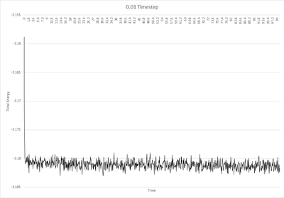
Since it is now known that the simulation reaches equilibrium at 0.01 timestep, longer timesteps can be trialed to find a more time efficient timestep. It is important to ensure that the timestep chosen for later experiments will also afford accurate results therefore simulations were ran at 4 further timesteps (0.0025, 0.0075, 0.01 and 0.15) and the total energy output from them were compared with that of the 0.01 timestep. It can be seen from Fig 5 that the total energy outputs from 0.0025 timestep are in very close agreement with those produced from 0.01 timestep. Systems simulated with 0.0075 and 0.01 both reach equilibrium but the output total energy values are slightly higher than those produced at the slowest timestep, 0.001, thus rendering them inaccurate. Therefore, the largest timestep that can be used to produce acceptable results is 0.025.The worst timestep to use would be 0.015 because the system does not reach equilibrium in the time simulated as indicated by the positive incline in total energy against time shown in Fig.5. Tick, what are you going to use and why?

Running simulations under specific conditions

The velocity Verlet algorithm allows for the observation of systems that preserve total energy(E), volume(V) and the number of atoms(N), also known as the NVE ensemble. In order to investigate molecular dynamics with different experimental conditions, the systems can be set up with different parameters to mimic those conditions. In this section, systems will be subject to the constant-pressure, constant temperature(NpT) and the constant volume ensemble.

Barostat and Thermostat

The energy of a molecule with N atoms, each with 3 degrees of freedom can be expressed as:

$E_K=\frac{3}{2}N{k}_{B}T$ (4)

$\frac{1}{2}\sum _i{m}_i{v}_i^2=\frac{3}{2}N{k}_{B}T$ (5)

The temperature will fluctuate after each timestep therefore a velocity-scaling constant, $\gamma$, is introduced to keep the system isothermal.

$\frac{1}{2}\sum _i{m}_i(\gamma v_i{)}^2=\frac{3}{2}N{k}_B\mathfrak{𝔗}$ (6)

To solve for $\gamma$, firstly, sum (5) and (6) to give

$\frac{1}{2}\sum _i{m}_i{v}_i^2+\frac{1}{2}\sum _i{m}_i(\gamma v_i{)}^2=\frac{3}{2}N{k}_{B}T+\frac{3}{2}N{k}_B\mathfrak{𝔗}$

Since $\gamma$ is a constant, it can be taken out of the summation and the equation can be rearranged to

$\frac{1}{2}\sum _i{m}_i{v}_i^2(1+{\gamma }^2)=\frac{3}{2}N{k}_B(T+\mathfrak{𝔗})$

Considering the relationship shown in eqn (5), the equation above can be rearranged to

$\frac{3}{2}N{k}_{B}T(1+{\gamma }^2)=\frac{3}{2}N{k}_B(T+\mathfrak{𝔗})$

$T(1+{\gamma }^2)=T+\mathfrak{𝔗}$

${\gamma }^2=\frac{\mathfrak{𝔗}}{T}$

$\therefore \gamma =\sqrt{\frac{\mathfrak{𝔗}}{T}}$ Tick

However, this is not the best method as rescaling at each step causes discontinuities in the momentum part of the phase space trajectory.

Examining the Input Script

 fix aves all ave/time 100 1000 100000 v_dens v_temp v_press v_dens2 v_temp2 v_press_2

the command "fix aves" applies the average operation to the systems. "ave/time 100 1000 100000" computes the global time-averages of the variables inputted(density, pressure and temperature). "100 1000 100000" specify the timesteps the input values will be used in order to contribute to the average. Therefore for this simulation, the final average will be calculated using values at timestep 100, 200, 300....100000. In total, 1000 values will be used to calculate the global average.

run 100000

This command tells LAMMPS to run the simulation over 100,000 timesteps. Since a timestep of 0.0025 will be used, 250 time units simulated. Why do you use variables?

Plotting the Equations of State

Fig.6:Density vs Time Graph at p=2.4 and p=2.6

The NpT ensemble (also known as the isothermal-isobaric ensemble) describes systems with a fixed number of particles, N, in contact with a thermostat at temperature $T$ and a bariostat *typo at pressure $p$. The system exchanges heat with the thermostat and pressure with the bariostat *barostat . Therefore, the total energy,$E$, and volume, $V$, both fluctuate at thermal equilibrium. Simulations were conducted at two pressures (2.4, 2.6 in reduced units), and at 5 temperatures(2, 2.5, 3, 3.5, 5). In order to compare the results obtained through the Lennard Jones simulations to theoretical Idea Gas Law ($PV=N{k}_{B}T$) results, a plot of density and temperature was constructed at both pressures(Fig.6). Good

In plot of density against temperature (Fig.6), the error bars of the data generated do not overlap, indicating that the density outputs from the simulations are statistically significant, thus analysis of the graphs can be carried out with confidence.

The graph shows density decreases with increasing temperature. This is an expected phenomenon as the system will increase in volume to compensate for the increase in kinetic energy due to increase in temperature. The Ideal Gas Law can be rearranged to show the inverse relationship between temperature and density.

$\frac{N}{V}=\frac{P}{k_{B}T}$ (7)

Fig.7: Graph of densities obtained through molecular modelling and Ideal Gas Law

Additionally, Fig.6 also shows that at constant temperature, density increases with increasing pressure. This is again expected because if increasing pressure was applied to a container with fixed number of particles, the volume would decrease, hence decreasing the density of the system. Again, this relationship can be justified by (7), where $\frac{N}{V}$ is directly proportional to $P$.

It can be seen from Fig.7 that the densities obtained through the Lennard-Jones molecular modelling is significantly lower than the densities obtained through Ideal Gas Law calculations. This is expected as the Ideal Gas Law assumes that molecules do not interact with each other, thus there will be no repulsion factor as there is in the LJ model, thus making the particles in the Ideal Gas system to be more compressible. This means that the molecules occupy negligible volume therefore for a given volume, the density will be higher. In the LJ model, the particles interact and repulsion occurs when $r$ is small, hence the density at a given volume will be lower. Tick

The Ideal Gas Law is most accurate in describing small gases at low pressure and low temperature

As seen from Fig.7, the largest discrepancies between the LJ simulation densities and the Ideal Gas densities occur at low temperature and high pressures(the gradient of Ideal Gas curve is higher at pressures whilst the gradient of the LJ simulation curve results do not differ as visibly). This is because the system behaves more like an ideal gas at high temperature and low pressure. The reason for this observation is that intermolecular interactions become less limiting when the thermal kinetic energy of the system is high i.e. high temperature; At lower pressure, assuming the volume is large, the intermolecular distance becomes larger therefore the density is less affected by the separation, $r$. Tick, very good

In conclusion, discrepancies increase with an increase in pressure and a decrease in temperature.

Heat Capacity Calculation

The NVT(canonical) ensemble describes systems have a fixed number of particles, N, and volume, V, that are in contact with a thermostat at temperature T. In this section, the heat capacities under the NVT ensemble were calculated for two different pressures (p=0.2 and p=0.8) and at five different temperatures each (T=2, 2.2, 2.4, 2.6, 2.8) by using the equation

$C_V=\frac{\partial E}{\partial T}=\frac{\mathrm{V}\mathrm{a}\mathrm{r}\left[E\right]}{k_B{T}^2}=N^2\frac{⟨E^2⟩-{⟨E⟩}^2}{k_B{T}^2}$(8)

To run the simulation under NVT conditions, the following code was used.

### DEFINE SIMULATION BOX GEOMETRY ###
variable dens equal 0.2
variable T equal 2.0
variable timestep equal 0.0025

lattice sc ${dens}
region box block 0 15 0 15 0 15
create_box 1 box
create_atoms 1 box

### DEFINE PHYSICAL PROPERTIES OF ATOMS ###
mass 1 1.0
pair_style lj/cut/opt 3.0
pair_coeff 1 1 1.0 1.0
neighbor 2.0 bin

### ASSIGN ATOMIC VELOCITIES ###
velocity all create ${T} 12345 dist gaussian rot yes mom yes

### SPECIFY ENSEMBLE ###
timestep ${timestep}
fix nve all nve

### THERMODYNAMIC OUTPUT CONTROL ###
thermo_style custom time etotal temp press
thermo 10

### RECORD TRAJECTORY ###
dump traj all custom 1000 output-1 id x y z

### SPECIFY TIMESTEP ###

### RUN SIMULATION TO MELT CRYSTAL ###
run 10000
unfix nve
reset_timestep 0

### BRING SYSTEM TO REQUIRED STATE ###
variable tdamp equal ${timestep}*100
variable pdamp equal ${timestep}*1000
fix nvt all nvt temp ${T} ${T} ${tdamp} 
run 100000
reset_timestep 0

### MEASURE SYSTEM STATE ###
thermo_style custom step etotal temp vol atoms
variable temp equal temp
variable temp2 equal temp*temps
variable energy equal etotal
variable energy2 equal etotal*etotal
variable atoms2 equal atoms*atoms
variable volume equal vol
fix aves all ave/time 100 1000 100000 v_temp v_temp2 v_energy v_energy2 v_volume
unfix nvt
fix nve all nve
run 100000

variable avetemp equal f_aves[1]
variable aveheatcap equal ${atoms2}*(f_aves[4]-(f_aves[3])(f_aves[3])f_aves[2]
variable avevolume equal f_aves[5]
variable aveheatcapv equal ${aveheatcap}/${avevolume}

print "Averages"
print "--------"
print "Temperature: ${avetemp}"
print "Total energy: ${etotal}"
print "Volume: ${avevolume}"
print "Heat Capacity: ${aveheatcap}"
print "Heat Capacity over V: ${aveheatcapv}"

The simulation box was defined with parameters of $15\times 15\times 15$ which resulted in a total of 3375 atoms. The volume for p=0.2 was and for p=0.8 was

In order to compare how heat capacities vary at different volumes, the heat capacity must be divided by the volume of each system thus $\frac{C_V}{V}$ was plotted against temperature for each system (Fig.8).

Fig.8: C_v/V against temperature for densities p=0.2 and p=0.8

The specific heat capacity defines how much heat is needed to raise the temperature of a unit mass by a unit degree of temperature. Fig.8 shows that the heat capacity has an inversely proportional relationship with temperature (so why the linear plot? ), in agreement with the definition of equation (8). This can be explained by the band-gap (density of states ) between the lattice energy levels decreasing with increasing temperature. Therefore, less energy is required to heat the system; relating this back to equation (8), where it is shown that $C_v$ is directly proportional to energy, increasing the temperature will decrease the heat capacity.

The results also show that heat capacity decreases with decreasing density. This is expected as high density leads to lower volume for a fixed number of atoms so it its expected that the heat required to raise the temperature of the system will be lower as particles are closer together compared to a lower density system with the same number of atoms where the volume is larger.Tick

Structural properties and the radial distribution function

The radial distribution function, g(r), describes the probability of finding a nearest neighbour from a reference particle. Thus it allows for the identification of the phase of the system as it provides information about the variation of density from a central reference particle. Tick

Fig 9 g(r) against distance for solid, liquid and gaseous phases

The radial distribution function was plotted for solid, liquid and gas for a Lennard-Jones material(Fig.9).The parameters were chosen from the Lennard-Jones phase diagram reported by Hansen and Verlet..

Phase	Density	Temperature
Solid	1.2	1.0
Liquid	0.8	1.2
Vapour	0.1	1.6

In all phases, a common factor was that g(r)=0 until r=0.9(reduced units). This is because at distances shorter than atomic diameter, strong repulsive forces causes the g(r) to be zero. Tick

The qualitative appearance for the three systems have clear differences. The solid system has the most number of peaks followed by liquid then vapour. This appearance is due to the fact that the peaks indicate the density around each reference atom therefore, the phase with the most regular structure,solids, will have the most discrete peaks. The solid peaks show a general decrease in amplitude as the r increases with some fluctuations (Why does it fluctuate?). The first three peaks in the solid RDF represent the first three coordination shells of the solid; the first peak represents the nearest neighbour of the reference molecule, the second peak is the second nearest neighbour and the third peak is the third nearest neighbour. There is zero probability of finding a particle in regions between the peaks as molecules in a solid cannot move. The distance between the zero probability minima gives the lattice spacing therefore the lattice spacing is defined by the second nearest neighbour; it is approximately 1.49 in reduced units. The appearance of the peaks in the solid system also indicate that the solid phase has long and short range order; the three tall peaks indicate short range order while the fluctuating smaller peaks indicate long range order.

The liquid g(r)has three peaks which decrease in amplitude with increased interatomic distance. The peaks are less narrow that those in the solid phase thus suggesting the system to have more disorder. The amplitude of the peaks decrease with separation, showing order decreases with separation due to the random Brownian motion of of particles. The low number of peaks in the radial distribution function suggests that there is only short range order in the system, specifically between the first three neighbouring atoms.

For gases, a single broad peak is observed at around r=1. The broad peak suggests that there is high disorder in the gaseous phase thus there is no short nor long range order. Tick

Fig.10: Expansion of the integral of g(r) for solid phase

Plotting the integral of the RDF against distance will give information about the coordination numbers of the neighbours of the reference particle in a solid. The inflection points called out in the Fig.10 show the coordination number of the three nearest neighbours of the reference particle. Since the solid system was modeled on a FCC lattice, the reference particle is expected to have 12 nearest neighbours (this is confirmed by the point at r=1.225). The next inflection point at r=1.625 has a g(r) integral of $\approx 18$. Since the plot is a running integral of g(r), the coordination number of the second nearest neighbours is $18-12=6$. Thus, the coordination number of the third nearest neighbours is $42-18=24$.Tick, nice

Dynamical properties and the diffusion coefficient

Mean Squared Displacement

The mean squared displacement measures the average distance a particle travels in a given time from a reference position, due to random motion. It is defined: $\mathrm{M}\mathrm{S}\mathrm{D}\equiv ⟨(x-x_0{)}^2⟩=\frac{1}{N}\sum _{n=1}^N(x_n(t)-x_n(0){)}^2$

In this equation, $x_n(t)-x_n(0)$ represents the vector distance traveled by a particle n over time interval of t. The square of the displacement is then averaged over N particles by summing n from 1 to N and then dividing by N.

Smaller system simulation(3375 atoms)	Larger system simulation(1 million atoms)
Fig.11a:Solid Simulation at d=01.2, T=1.0	Fig.11b:Solid Simulation at d=0.8, T=1.2
Fig.12a:Liquid Simulation at d=0.8, T=1.2	Fig.12bLiquid Simulation at d=0.8, T=1.2
Fig.13a:Vapour Simulation at d=0.1, T=1.6	Fig.13b:Vapour Simulation at d=0.1, T=1.6

The plots generated are shown above. In a solid system, the particles are bound to their position so there is not sufficient kinetic energy to reach a diffusive behaviour and this is shown in Fig.11a, as indicated by the nearly constant value of the MSD after around timestep 200.

The liquid plot(Fig.12) shows a clear linear relationship ($R^2=0.9999$) between MSD and time. This shows that the particles in the system move acccording to Brownian motion.

Fig.14:Vapour Simulation at d=0.1, T=1.6 for smaller system at timesteps above 2000

In the plot for the gaseous phase(Fig.13), relationship between MSD and time is initially curved, followed by a near linear relationship(shown by Fig.14 when only consdiering the relationship between MSD and time above timestep 2000). The inital curvation is due to the fact that atoms are placed randomly to simulate the system. Since it is a gaseous system, the interatomic separations are high. This results in a lower frequency of collisions thus the overall velocity the atoms travel at appears to be constant. Therefore, by definition, the distance travelled per unit time is also constant, hence MSD is proportional to $t^2$. As more time is simulated, more collisions occur and the atomic motion becomes more consistent with Brownian motion thus the MSD/Time graph tends to linearity. Takes a while for the system to act like a random walk

The simulations performed at 3375 atoms and a million atoms both generated MSD/Time graphs that show the same general trends for each phase. In the solid simulations, there is less fluctuations in the MSD of the larger system, suggesting the system to be more stable for solids. The difference in the output values of simulation performed on 3375 atoms and the 1 million atoms are relatively small(around 0.02 difference in MSD). Since the phase parameters used for the larger simulation were not stated, the discrepancy could also be caused by the different simulation conditions used. However, this discrepancy could also be due to the difference in number of atoms used; if this were the case, it can concluded that there is no need to use such large systems as the difference in output data is not significantly difference thus the tradeoff for longer simulation times is not worthwhile. Tick

Einstein showed that the the self-diffusion coefficient is related to the mean-squared displacement:

$D=\frac{1}{6}\frac{\delta ⟨r^2⟩}{\delta t}$

Substituting simulation values for the 3375 atoms system, the diffusion coefficients in reduced units are

Gas:$D=\frac{1}{6}\times \frac{0.0226}{0.002}=1.88$ Solid: $D=5.00\times 10^{-5}$ Liquid:$D=8.33\times 10^{-2}$

For the larger 1 million atoms system

Gas:$D=\frac{1}{6}\times \frac{0.0326}{0.002}=3.03$ Solid: $D=4.17\times 10^{-7}$ Liquid:$D=8.33\times 10^{-2}$

The diffusion coefficients are very similar for the smaller and larger model.Tick

Velocity Autocorrelation Function

The motion of a 1D harmonic oscillator is given by

$x(t)=A\cos (\omega t+\varphi )$

Velocity is the first derivative of positions and time:

$v(t)=\frac{dr}{dt}$

Therefore, the position of a 1D harmonic oscillator at a specific velocity can then be found by substituting

$v(t)=\frac{d(Acos(\omega t+\varphi )}{dt}$ $v(t)=-A\omega sin(\omega t+\varphi )$

At timestep t+\tau , the velocity will therefore be:

$v(t+\tau )=-A\omega sin(\omega (t+\tau )+\varphi )$

Substituting this into the velocity correlation function,

$C(\tau )=\frac{\underset{-\mathrm{\infty }}{\overset{\mathrm{\infty }}{\int }}A\omega sin(\omega t+\varphi )A\omega sin(\omega (t+\tau )+\varphi )\mathrm{d}t}{\underset{-\mathrm{\infty }}{\overset{\mathrm{\infty }}{\int }}(-A\omega sin(\omega t+\varphi ){)}^2\mathrm{d}t}$

$C(\tau )=\frac{\underset{-\mathrm{\infty }}{\overset{\mathrm{\infty }}{\int }}sin(\omega t+\varphi )sin(\omega (t+\tau )+\varphi )\mathrm{d}t}{\underset{-\mathrm{\infty }}{\overset{\mathrm{\infty }}{\int }}si{n}^2(\omega t+\varphi )\mathrm{d}t}$

Considering the trigonometric identity $sin(x+y)=sin(x)cos(y)+cos(x)sin(y)$. The equation can therefore be written as:

$C(\tau )=\frac{\underset{-\mathrm{\infty }}{\overset{\mathrm{\infty }}{\int }}sin(\omega t+\varphi )[sin(\omega t+\varphi )cos(\omega \tau )+cos(\omega t+\varphi )sin(\omega \tau )]\mathrm{d}t}{\underset{-\mathrm{\infty }}{\overset{\mathrm{\infty }}{\int }}si{n}^2(\omega t+\varphi )\mathrm{d}t}$

Since $\omega$ and $\tau$ are both constants, they can be taken out of the integral:

$C(\tau )=\frac{cos(\omega \tau )\underset{-\mathrm{\infty }}{\overset{\mathrm{\infty }}{\int }}si{n}^2(\omega t+\varphi )}{\underset{-\mathrm{\infty }}{\overset{\mathrm{\infty }}{\int }}si{n}^2(\omega t+\varphi )\mathrm{d}t}+\frac{sin(\omega \tau )\underset{-\mathrm{\infty }}{\overset{\mathrm{\infty }}{\int }}sin(\omega t+\varphi )cos(\omega t+\varphi )\mathrm{d}t}{\underset{-\mathrm{\infty }}{\overset{\mathrm{\infty }}{\int }}si{n}^2(\omega t+\varphi )\mathrm{d}t}=cos(\omega \tau )+\frac{sin(\omega \tau )\underset{-\mathrm{\infty }}{\overset{\mathrm{\infty }}{\int }}sin(\omega t+\varphi )cos(\omega t+\varphi )\mathrm{d}t}{\underset{-\mathrm{\infty }}{\overset{\mathrm{\infty }}{\int }}si{n}^2(\omega t+\varphi )\mathrm{d}t}$

Since $sin(x)$ is an odd function, evaluating its integral by limits that are symmetric across the origin,$-\mathrm{\infty }$ to $\mathrm{\infty }$, will be zero. Thus the right hand side of the equation will equal zero and the equation becomes:

$C(\tau )=cos(\omega \tau )$

Good

Fig.15: Graph of VACF for solid, liquid and the Simple Harmonic Oscillator

A graph of VACF for the Lennard Jones liquid and solid simulations was plotted along with the VACF graph of the Simple Harmonic Oscillator. It can be observed in the graph that there is a maximum difference between the $\nu (t)$ and $\nu (t+\tau )$ at the minima of the solid and liquid plots. In the solid,, this indicates that atoms have collided and are changing directions of motion. In the liquid, this phenomena can be attributed to the atom colliding with their "solvent cage" and then changing direction. The minima of the solid is lower than the minima of the liquid as there are stronger interatomic forces in the solid. Tick, nice description

The liquid VACF has one weak oscillation as the particles in the system only interact with their closest neighbours whereas in the solid, a series of oscillations are seen as the ordered lattice allows atoms to vibrate forwards and backwards. However, the amplitude of the oscillations become smaller.

For the Simple Harmonic Oscialltor, the appearance of the VACF is very different. This is due to the fact that the oscillator does not consider the interactions with other atoms in the system, and instead models a system with no energy loss, thus the velociy never decreases.

To find the running integral of under the VACF graphs, the trapezium rule was employed as the diffusion coefficient can also be defined as

$D=\frac{1}{3}\underset{0}{\overset{\mathrm{\infty }}{\int }}\mathrm{d}\tau ⟨\mathbf{v}\left(0\right)\cdot \mathbf{v}\left(\tau \right)⟩$

The last point of data on the running integral of VACF graphs gives the total integral of the VACF graphs.

For the smaller system the results are as follows

Fig.16a:Running intergral of VACF against time for Gas in small system

Fig.16b:Running intergral of VACF against time for Liquid in small system

Solid:$D=4.63\times 10^{-4}$

Liquid:$D=7.93\times 10^{-2}$

Gas:$D=2.35$ Tick

Fig.18a:Running intergral of VACF against time for Gas in large system

Fig.18b:Running intergral of VACF against time for Liquid in large system

For larger system, the diffusion coefficients are

Solid:$D=5.67\times 10^{-5}$

Liquid:$D=7.93\times 10^{-}2$

Gas:$D=2.35$

There is little discrepancy with the diffusion coefficients obtained from the larger and smaller system.

The coefficients calculated from the VACF method show the same trend as the Mean Displacement Squared approach. The diffusion coefficient was largest for gases, then liquids and smallest for solids. Neither methods were particularly affected by the sample size of the simulation box. The two methods produced $D$ of similar values and of similar magnitudes for the liquid and gas simulations but the coefficients from the VACF method were larger significantly larger than those obatined thorugh the MSD method. Therefore, it must be noted that using the trapezium rule to integrate the VACF is likely to accumulate errors over time, especially for solids as solid VACF curves are non periodic. The accuracy of the method could be increased by using smaller timesteps but this would have implications on the simulation time. Another way to refne the VACF method would be to use a more sophisticated integration method. Good comparison