Talk:ModMonteCarlo:K98631
JC: General comments: Some good explanations and extra analysis, however, take more care to read the experiment instructions and check your code. Writing your report as you go along might help to make sure that it follows the order of tasks in the instructions.
Peter Wright 3rd year CMP python- Monte Carlo simulation report
Introduction to the Ising model
a) In the Ising model we consider a lattice, of variable dimension D, with N spins arranged on individual lattice domain sites, with spins si,j=+-1.For a configuration ‘v’, the total interaction energy due to spin interaction, J can be written using the following equation;

J is a spin-coupling constant, and interactions occur between neighboring spins. Periodic boundary conditions are set such that the lattice site at the end of a row/column interacts with the lattice site at the opposite end. This happens in both directions. Parralel spins have a –J interaction and opposing spins have no energetic interaction.
Because J>0, spin alignment is energetically favorable, and hence spin alignment is favoured. Below the Curie temperature; where the energetic component of the systems free energy is dominant, we expect spontaneous magnetization, leading to long-range ordering of spins. The lowest energy ground state of the system has E=-DNJ.
This is shown by considering a generous square 2D lattice; the total number of edges= 4N/2, or 2N if there are N sites. As the ground equilibrium state of the lattice correspond to either all spins being +1(up) or -1(down), i.e in the same state, the ground state energy will be –J for each edge. Every spin, in an nxn lattice of dimensionality D, is connected to its neighbor by 2D (four) edges, so the total contribution, taking into account periodic boundary conditions is -4NJ/2. The factor of 0.5 is to account for double counting that occurs when cycling through each lattice site as each edge appears twice in the sum. Therefore for dimensionality D, the ground state energy= -DNJ.
b) For an nxn lattice consisting of N=1000 spins, and D=3. If we consider the lattice to be in its ground state, whereby E=-DNJ, and we now randomly flip one spin such that it is now aligned oppositely to all other lattice spins, the system configuration will increase in energy.
As D=3, each lattice site has 6 edges, therefore when a single spin is flipped the total number of energetically favorable interactions lost is +6J. This does not propagate as the system wants to minimize the energy loss, and it would be rare, due to Boltzmann probability that this new configuration would be adopted. Nevertheless, for the lattice in question; = -2994J - -3000J = +6J. This spin flipping leads to greater system disorder, which is entropically favorable. The ground state configuration, which is favoured at T<TC, has only one ‘microstate (w)’ or permutation, and therefore the third law of thermodynamics; S=KBIn(0) = 0. The new, higher energy configuration has N lattice permutations, and therefore S=KBIn(1000) ≈ 9.54x10⁻²³JK-1mol-1.
JC: When a spin is flipped in the ground state configuration, 6J favourable interactions are lost and 6J unfavourable interactions are gained, so the total change in energy for flipping one spin in 12J (remember parallel spins have a favourable interaction -J and antiparallel spins have an unfavourable interaction +J). The ground state has a multiplicity of 2 as all spins can be up or down, so S = 9.57e-24 J K-1. The single spin flipped state has a multiplicity of 2N as any one of the N spins can be flipped and can either be pointing down with all other spins pointing up or vice versa. Also note that ln(0) != 0, ln(0) is undefined because ln(x) -> infinity as x -> 0.
This was also shown using calculations made in python- source code found below for 1, 2 and 3D lattices. (EXTRA CODE, JUST FOR DEMONSTRATION)
<code>
import numpy as np
f = lambda x, y : 1 if np.sign(x) == np.sign(y) else 0
J = -1;
D = 3; N = 3; dim = np.array([N] * D); e_min=0; a_min = np.zeros(N ** D); a_min = np.reshape(a_min, dim)
for k in range(1):
a = np.random.choice([-1,1],N ** D); a = np.reshape(a, dim)
a = np.ones(N ** D); a[0] = -1
a = np.reshape(a, dim)
if D == 1: b = a; d = [[f(j, b[i-1]) + f(j, b[(i+1) % N]) for i,j in enumerate(b)]]
if D == 2:
d1 = [[f(j, b[i-1]) + f(j, b[(i+1) % N]) for i,j in enumerate(b)] for b in a]
d2 = [[f(j, b[i-1]) + f(j, b[(i+1) % N]) for i,j in enumerate(b)] for b in a.T]
d = np.sum(d1) + np.sum(d2)
if D == 3:
c = a
d1 = [[[f(j, b[i-1]) + f(j, b[(i+1) % N]) for i,j in enumerate(b)] for b in a] for a in c]
d2 = [[[f(j, b[i-1]) + f(j, b[(i+1) % N]) for i,j in enumerate(b)] for b in a.T] for a in c]
d3 = [[[f(j, b[i-1]) + f(j, b[(i+1) % N]) for i,j in enumerate(b)] for b in a] for a in c.T]
d = np.sum(d1) + np.sum(d2) + np.sum(d3)
e = 0.5 * J * np.sum(d)
if e < e_min: e_min = e; a_min = a
print(e_min, a_min)
</code>
It is shown that a single spin flip, leads to an energy change of +2DJ.
JC: You are not calculating the energy correctly in this code, see below. Also try to present your code in a different font to the rest of the text so that it is easy to see which lines are code.
c) A lattices total magnetization is calculated via a simple sum of all lattice site spins;
Figure 1 PNG (see CMP Intro to Ising Lattice page1).
1D- 3up spins and 2 down spins = +1
2D- 13up spins and 12 down spins= +1
At absolute zero, T-0K, thermal energy available to a lattice, KBT=0J. Considering this, the lattice cannot flip a spin in order to reach a higher energy configuration other than its ground state. Furthermore there will be no entropic contribution to the free energy, making the process impossible. Therefore a lattice, D=3 and N=1000; all spins will be in the same state.
=+1000 or -1000.
JC: Magnetisations are correct.
Calculating the energy and magnetisation
Working in reduced units, where J=KB python IsingLattice functions are completed. Source code found below.
<code>
def energy(self):
"Return the total energy of the current lattice configuration."
f = lambda x, y : 1 if np.sign(x) == np.sign(y) else 0 #lamdba function to compute energy of interaction between neighbours x and y
J = 1
d1 = [[f(j, b[i-1]) + f(j, b[(i+1) % self.n_rows]) for i,j in enumerate(b)] for b in self.lattice] #enumerate rows and calculate energy with modulus calc on index to satisfy the periodic boundary condition
d2 = [[f(j, b[i-1]) + f(j, b[(i+1) % self.n_cols]) for i,j in enumerate(b)] for b in self.lattice.T] #enumerate columns (transpose) and calculate energy
d = np.sum(d1) + np.sum(d2) #add row and column energies
energy = 0.5 * J * np.sum(d) #0.5 factor adjusts for double counting in neighbour interactions
return energy
def magnetisation(self):
"Return the total magnetisation of the current lattice configuration."
j = 0
for i in np.hstack(self.lattice): #use hstack to vectorise matrix and enumerate through each element and accumulate total
j += i
return j
</code>
JC: You are not calculating the energy correctly. In your code the energy of a pair of antiparallel spins is 0, but if you look at the energy equation for the Ising model, the energy for a pair of antiparallel spins in +J. You are also missing the minus sign at the start of the Ising model energy equation. Using the remainder "%" operator to deal with the periodic boundary conditions is nice idea. Your magnetisation function is correct.
Functions are tested to ensure they work using the ILCheck.py script.
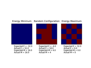
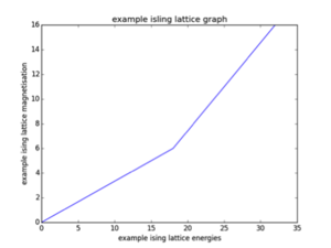
JC: You can see from the output of the ILCheck.py script that there is a problem with your energy function as the "Expected" and "Actual" energy do not agree. This is because you are not including the +J contribution to the energy from antiparallel spins.
Introduction to Monte Carlo simulation
a) A lattice system of 100 spins, where each can either be in the +1 or -1 state has 2100 possible configurations or approximately 1.268x1030. This is a lot of configurations to analyse. For example if we consider that our computer can analyse 1x10⁹ configurations per second, to evaluate an average value such as that of <M>T over all the configurations would take roughly 1.269x10²¹ seconds to analyse. This is obviously not feasible and we need to consider a way to prioritise configurations that can actually be formed. Most of the configurations will be of a high energy, if we consider a ground state lattice the probability of obtaining these configurations is given by the Boltzmann statistical thermodynamic probability. This factor will become very small for high-energy configurations. We can consider ‘importance sampling’ and the Monte-Carlo simulation, which filters out configurations where the Boltzmann factor is very small, according to its probability weighing.
JC: The number of possible configurations and time taken are correct, however, it would be good to write the time taken in a more intuitive unit, e.g. years.
b) MonteCarloStep(T) and statistics() functions are completed see source code below.
<code>
def montecarlostep(self, temperature):
# complete this function so that it performs a single Monte Carlo step
#the following two lines will select the coordinates of the random spin for you
random_i = np.random.choice(range(0, self.n_rows))
random_j = np.random.choice(range(0, self.n_cols))
E0_energy = self.energy()
E0_magnetisation = self.magnetisation()
self.lattice[random_i, random_j]*=-1 #flip the randomly selected lattice site
E1_energy = self.energy()
E1_magnetisation = self.magnetisation()
energy_diff = (E1_energy - E0_energy)
if energy_diff <= 0: #accept new configuration if lower energy
E0_energy = E1_energy
E0_magnetisation = E1_magnetisation
elif energy_diff > 0:
#the following line will choose a random number in the rang e[0,1) for you
random_number = np.random.random()
if random_number <= np.exp(-1 * energy_diff / (temperature)): # if new config is higher then do Boltzmann test to determine whether to accept a higher energy state with probability exponentially decaying with respect to the energy difference
E0_energy = E1_energy
E0_magnetisation = E1_magnetisation
else:
self.lattice[random_i, random_j] *= -1 #else reject new higher energy configuration
self.n_cycles += 1
if self.n_cycles > 2000: #ignore first 2000 cycles which corresponds to the equilibriating period- starting from a purely random state is not a realistic physical state
self.equicycles += 1
self.E += E0_energy
self.E2 += (E0_energy ** 2)
self.M += E0_magnetisation
self.M2 += (E0_magnetisation ** 2)
return E0_energy, E0_magnetisation
def statistics(self):
self.AE = self.E/self.equicycles
self.AE2 = self.E2/self.equicycles
self.AM = self.M/self.equicycles
self.AM2 = self.M2/self.equicycles
return self.AE, self.AE2, self.AM, self.AM2, self.equicycles
# complete this function so that it calculates the correct values for the averages of E, E*E (E2), M, M*M (M2), and returns them
</code>
Functions are tested using ILanim.py scipt and three outputs were validated with outputs just after the system T=1<Tc , L=8x8, reached its expected ground state equilibrium.

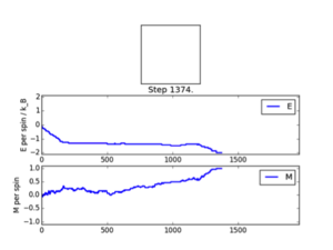

JC: Your Monte Carlo code is correct. However, at this point you are not asked to take equilibration into account. Your ploted simulations and statistics do not reach 2000 steps so must have been generated with a Monte Carlo function without accounting for the equilibration period.
Observations: It can be seen that the system reached its expected equilibrium state where all spins are aligned. The number of MonteCarlosteps() function runs needed in order to reach this state varied from 563-1374. This is explained via the randomness factor incorporated in the montecarlostep() function, whereby a np.random number between 0-1 is selected and then tested against <= the energy change of configurations incorporated in its Boltzmann probability; Furthermore the systems initial state is a randomly configured numpy array and has no physical meaning. The ‘random walk’ toward the ground state is therefore bound to vary due to these two factors. However reaching this state validates the functions.
This was expected as when T<Tc spontaneous magnetization occurs. This physical phenomenon is explained by thermodynamics as the Curie temperature represents the highest temperature at which non-zero magnetization occurs. It represents a phase transition point for the Ising Lattice at which the energetic and entropic driving forces of free energy are balanced. ; Below Tc the energetic factor dominates and it is therefore favourable for spins to be aligned to produce to maximum number of spin interactions and hence minimise system disorder and have spontaneous magnetization. However above which the entropic factor dominates and disorder is favoured leading to domain misalignment and a tendency to zero lattice magnetisation, as checkerboard spins lead to maximum disorder and a new equilibrium for the system is observed and an energy minimum=0, is observed.
JC: Good explanation of the interplay between energy and entropy in controlling the properties of the Ising model either side of the Curie temperature.
Accelerating the code
Both energy() and magnetisation functions are re-coded.
Energy()- Using a for loop and enumeration inside the python interface to using a numpy.roll function. This is significantly quicker as it utilises an internal function within python, compiled in C++, a much lower level language. Instead of looping through each lattice site and counting the number of interactions with neighbours individually, the roll function allows the user to quickly measure all lattice site interactions simultaneously. Furthermore I have demonstrated the possibility of avoiding lattice-site double counting. Each roll either along a row/column (row.T), already takes into account two neighbouring edges interactions. The comparion can be seen in the source code evolution……..
Magnetisation()- Again a python for loop is replaces, this time with a simple np.sum of the array output from the lattice. The comparison can be seen in the source code evolution; Note the when utilising the roll function, it was found that two rolls were adequate as these account for neighbouring site interactions, without double-counting (old code commented out)
<code>
def energy(self):
"Return the total energy of the current lattice configuration."
#roll1 = np.roll(self.lattice, 1, axis = 1) #use bumpy roll in place of inefficient enumeration in base python
#roll2 = np.roll(self.lattice, -1, axis = 1)
#roll3 = np.roll(self.lattice, 1, axis = 0)
#roll4 = np.roll(self.lattice, -1, axis = 0)
#mult1 = np.multiply(self.lattice, roll1) #efficiently compute energy of neighbour interaction by matching up neighbours and multiplying energy states (neighbours with same sign give a 1 and neighbours with different signs -1) - we can then sum positive results to compute the energy
#mult2 = np.multiply(self.lattice, roll2)
#mult3 = np.multiply(self.lattice, roll3)
#mult4 = np.multiply(self.lattice, roll4)
#energy = -0.5 * J * (np.sum(mult1[mult1>0]) + np.sum(mult2[mult2>0]) + np.sum(mult3[mult3>0]) + np.sum(mult4[mult4>0]))
target_energy = -1.0*np.sum(np.multiply(self.lattice, np.roll(self.lattice, 1, 0))) #more efficient approach that eliminates 2 rolls and 2 multiplies and avoids the double counting of neighbour interactions
target_energy -= 1.0*np.sum(np.multiply(self.lattice, np.roll(self.lattice, 1, 1)))
energy = target_energy
#d = np.sum(d1) + np.sum(d2)
#energy2 = 0.5 * J * np.sum(d)
return energy
def magnetisation(self):
"Return the total magnetisation of the current lattice configuration."
return np.sum(self.lattice)
</code>
JC: Good use of numpy functions to accelerate the code and well noticed that you only have to perform 2 rolls, rather than 4.
The ILtimetrial.py scipt is utilised to quantitatively determine the length of time the computer took to run 2000 MonteCarlo cycles. The results were determined within a 30min time frame in order to minimise error, due to varying CPU usage throughout the day. The results for the individual, and combined function accelerations, the average, and the error involved in these measurements are presented below; each trial included 10 repeat runs [See Appendix].
|
Average time (s) |
Standard Deviation |
Standard Error | |
|
Slow E(), Slow M() |
64.2217106 |
0.190598169129 |
0.0602724332306 |
|
Slow E(), Fast M() |
63.6513610 |
0.248100941936 |
0.078456406615 |
|
Fast E(), Slow M() |
2.12632640 |
0.00857236824791 |
0.00271082086051 |
|
FAST E(), Fast M() |
1.11812940 |
0.00750646746627 |
0.00237375343754 |
As can be seen the major acceleration was due to the energy() function. This increase is approximately x30.2, compared to magnetisation()’s x1.009. This difference is significant and can be attributed to the fact that the original energy function required two extensive for loops and calculation of interactions, whereas the original magnetisation function had only one for loop and no enumerate operator.
JC: Great idea to investigate what effect that the new accelerated code has on the speed of the energy and magnetisation functions individually.
The effect of temperature
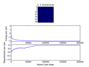
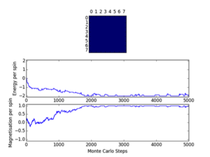
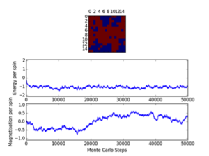
a) The IsingLattice model used so far, originally starts from a random lattice nxn configuration. This configuration has no physical meaning. When running the ILanim.py script is can easily be seen that below Tc, which decreases with increased lattice size (2D), after a certain number of runs tends to an equilibrium state where all spins are aligned, either up, or down with total energy being equal to the minimum ground state, E=-DNJ whereby energy per spin=-2, and magnetisation per spin =. Furthermore it was seen when T>Tc, whereby system disorder and domain disaligment is favoured that a new equilibrium state is reached; total energy(/spin) and magnetisation per spin both equal to zero. Both of these states are equally valid physical states of the Ising Lattice. It can also be seen from the IL.Finalframe that in the energy and magnetisation per spin plots vs. number of MC cycles that this equilibrium stage takes a certain number of runs to reach. Beforehand the system was in a physically meaningless random state and is in an equilibrating period. To study the systems physical behaviour we opt to ignore data corresponding to this region using self.equicycles counter seen. This is seen in the MonteCarloStep() and statistics() function's in the Monte-Carlo intro section.


Cutoff; 8x8; <500/480/750, 16x16; <7100/10000/9700, 32x32; <15000


Cutoff; 8x8; <370/900/650, 16x16; <6300/10200/9500, 32x32; <20000

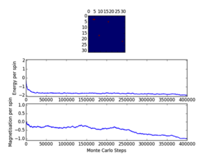
Cutoff; 8x8; <1800/1400/1400, 16x16; <12000/13500/15000, 32x32; <25000


Cutoff; 8x8; <1250/2050/1000, 16x16; <25000/14000/15000, 32x32; <75000
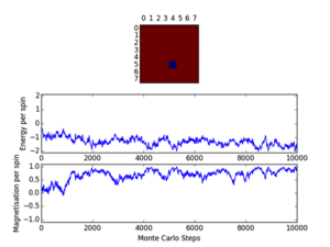
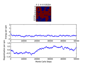

Cutoff; 8x8; <2100/2000/1400, 16x16; <2000, 32x32; <10000
Three repeats were undertaken for each lattice size at each temperature in order to validate any trends using the ILfinalframe.py script. Two trends are immediately seen; as lattice size increases the number of cycles taken to reach a physical state equilibrium increases. This is due to the random initial configuration and, how via the MonteCarlo simulation a random walk is assigned in order to reach these states. For more lattice sites this will take longer as there are more spins to flip and test. This generally leads to an increase in the order of magnitude of steps needed in order to reach equilibrium, this is only seen for T<Tc. This is because above the Curie temperature the randomly assigned initial configuration is very near the actual physical disordered equilibrium state, and therefore easy to reach via a random walk. However below this, the number of cycles taken in the equilibrating period behaves extensively in relation to the lattice size. Secondly once the lattice systems have reaches equilibrium the fluctuations above the equilibrium values increase with temperature. As a result of this analysis a cut-off point of 4500 cycles was assigned and implemented in the MonteCarloStep() function using an if statement relation the no. of cycles elapsed to ones >4500, and only these would be taken into account in the average data in the statistics() function. This number would eliminate the main source of error because for the maximum lattice size analysed, 32x32, where the variation is a maximum, this cut-off value is feasible and therefore is for smaller lattices by virtue of a lesser number of spins needing to be flipped. Moreover 150000 cycles are taken for averages such that any error would be diluted in output averages.
JC: Well noticed that number of cycles needed to reach equilibrium increases with system size. Is using a cut-off of 4500 cycles really enough to ensure that you system has reached equilibrium before you start calculating statistics?
Furthermore it should be noted that metastable states do form and can last for upwards of 10000 cycles and increase in likelihood with lattice size. Because once one starts to form starts it can be very hard to flip back, especially at large lattice sizes where it’s less probable as there are more possibilities geometrically for regions to form and be closed in at the edges ie. DeltaE=8J to change=unlikely.. These states seem to be temperature independent as they occurred at low and well as T>Tc. Tc appears to occur around T=2.0K as entropic and energetic driving forces are most balanced here leading to larger numbers of cycles being needed to reach equilibrium than at other temperatures. This observation is validated by the later result that Tc is around 2.24K.
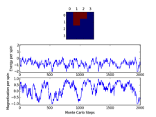
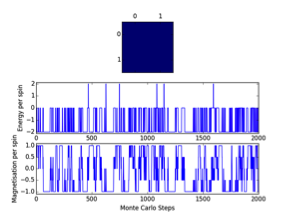
Furthermore 2x2 and 4x4 lattices were analysed even though they are too finite for useful results. In general the Curie temperature appears earlier and the same overall trends occur as for the other lattices, for plots [Appendix].
These states do have physical meaning, but will interfere with averaging data and are a source of error. Some examples of these include; T=0.5K (8x8, 32x32) and T=2.5K (32x32), these are local minima, not equilibrium states of the system.


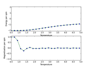
b) a) ILtemperaturerange.py scipt utilised to run 150000 MonteCarlo cycles over a temperature range (0.5, 5.0, 0.1), with error bars to determine size of error and validate the cutoff point of 4500 for an 8x8 lattice. The data outputs are then saved using np.savetxt(“”, final_data) where final data contains 5 volumns; energy per spin, energy per spin squared, magnetisation per spin, magnetisation per spin squared and variance per spin. The output is shown below. This demonstrates the phase transition at around T=2.2K where energy/s tends from -2 to 0, and magnetisation per spin tends from +1 to 0. This demonstrates graphically the two physical equilibrium states of the Ising Lattice, one for ferromagnetic energetic spin alignment, and T>Tc where entropic disorder of a paramagnet is favoured. The 8x8 lattice size plot is shown below. Furthermore error bars are plotted (updated ILtemperaturerange source code next section). I determined that each simulation should be 150000 cycles as this would lead to a lot of post-cutoff data that when averaged would dilute any errors.
JC: Plots look good, but cannot see error bars.

Scaling the system size
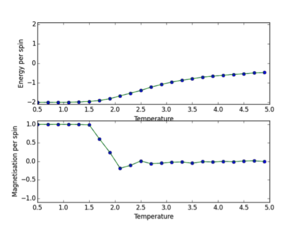
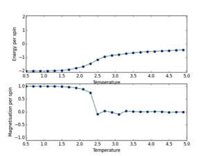
This process was repeated for L=2, 4, 16, 32, in order to obtain the output data in a .data file for all lattice sizes under analysis. A Python script to make a plot showing the energy per spin versus temperature for each of your lattice sizes, whereby the numpy.loadtxt function was utilized to read and index the column data in the files and plot the energy per spin vs. temp and magnetization per spin vs. temp for all lattice sizes.
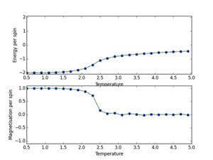
<code>
from IsingLattice import *
from matplotlib import pylab as pl
import numpy as np
n_rows = 8
n_cols = 8
il = IsingLattice(n_rows, n_cols)
il.lattice = np.ones((n_rows, n_cols))
spins = n_rows*n_cols
runtime = 150000
times = range(runtime)
temps = np.arange(0.5, 5.0, 0.2)
energies = []
magnetisations = []
energysq = []
magnetisationsq = []
for t in temps:
for i in times:
if i % 100 == 0:
print(t, i)
energy, magnetisation= il.montecarlostep(t)
aveE, aveE2, aveM, aveM2, n_cycles = il.statistics()
energies.append(aveE)
energysq.append(aveE2)
magnetisations.append(aveM)
magnetisationsq.append(aveM2)
#reset the IL object for the next cycle
il.E = 0.0
il.E2 = 0.0
il.M = 0.0
il.M2 = 0.0
il.n_cycles = 0
il.equicycles = 0
yerr = ((((np.array(energysq) - np.array(energies)**2)**0.5)/spins)/(n_cycles**0.5)) #error determination for error bars
yerr2 = ((((np.array(magnetisationsq) - np.array(magnetisations)**2)**0.5)/spins)/(n_cycles**0.5))
fig = pl.figure()
enerax = fig.add_subplot(2,1,1)
enerax.set_ylabel("Energy per spin")
enerax.set_xlabel("Temperature")
enerax.set_ylim([-2.1, 2.1])
enerax.errorbar(temps, np.array(energies)/spins, yerr, fmt='--o')
magax = fig.add_subplot(2,1,2)
magax.set_ylabel("Magnetisation per spin")
magax.set_xlabel("Temperature")
magax.set_ylim([-1.1, 1.1])
magax.errorbar(temps, np.array(magnetisations)/spins, yerr2, fmt='--o')
enerax.plot(temps, np.array(energies)/spins)
magax.plot(temps, np.array(magnetisations)/spins)
pl.show()
Var_ET = ((np.array(energysq) - np.array(energies)**2)/(temps**2))
print(spins)
print(energies)
print(magnetisations)
print(np.array(energysq)/(spins**2))
print(magnetisationsq)
final_data = np.column_stack((temps, (np.array(energies)/(spins)), (np.array(energysq)/(spins**2)), (np.array(magnetisations)/(spins)), (np.array(magnetisationsq)/(spins**2)), (Var_ET/(spins))))
np.savetxt("8x8NEW2.dat", final_data)
</code>
From these graphs it can be seen that the error bars are extremely small, this shows the variation in my data points due to initial equilibrating-state data values are insignificant and the cut-off point is justified. Furthermore these lattice sizes follow the same general phase transition trend as for the 8x8 lattice. However it can be seen that as the lattice size increases the point of transition tends to higher temperature values.
These lattice size data plots are easily compared utilising the following plot;
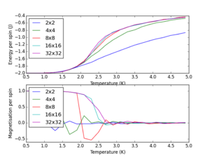
From this plot it is obvious that lattice sizes 2x2 and 4x4 are too small to give reasonable results, and this is also seen in the linear regression to determine the Tc for an infinite lattice. Phase transition theory states that an infinite system is required, in a system like this the heat capacity diverges to infinity and becomes discontinuous. The plot above shows the region where the finite lattices converge to resemble infinite systems behaviour. This happens as the length of the 2D lattice becomes 8 and continues for 16x16 and 32x32 systems. Therefore the minimum lattice size needed to capture long-range fluctuations is 8x8. Data obtained for intermediate lattice sizes would help to pinpoint the exact length at which this behaviour starts to occur.
JC: Good analysis of the system size dependence and identification of the 8x8 system as the minimum system size able to capture long range fluctuations.
This required using the np.savetxt() function to import my data and superimpose the plots ontop of each other, source code as follows;
<code>
from IsingLattice import *
from matplotlib import pylab as pl
import numpy as np
a = np.loadtxt("2x2NEW.dat")
b = np.loadtxt("4x4NEW.dat")
c = np.loadtxt("8x8NEW.dat")
d = np.loadtxt("16x16NEW.dat")
e = np.loadtxt("32x32NEW.dat")
j = [a, b, c, d, e] # incorporates imported data into a list
fig = pl.figure()
for i in j:
enerax = fig.add_subplot(2, 1, 1)
enerax.set_ylabel("Energy per spin (J)")
enerax.set_xlabel("Temperature (K)")
magax = fig.add_subplot(2, 1, 2)
magax.set_ylabel("Magnetisation per spin")
magax.set_xlabel("Temperature (K)")
enerax.plot(i[:, 0], i[:, 1]) # indexing relevant colums from data, 1st col temp, 2nd energy per spin
magax.plot(i[:, 0], i[:, 3]) # as above, but 3rd column magnetisation per spin
enerax.legend(['2x2', '4x4', '8x8', '16x16', '32x32'], loc='upper left')
magax.legend(['2x2', '4x4', '8x8', '16x16', '32x32'], loc='upper left')
pl.show()
JC: Good use of the loadtxt function.
</code>
Furthermore we can now conclusively talk about the qualitative behaviour of our Ising Lattice.
T<Tc; Low temperature ferromagnetic phase. There is a dominance of one spin throughout the Monte-Carlo cycles e.g. si = +1. Also flucuations of the other spin occurring only happens in isolated clusters. These increase in frequency with lattice size, but the system always tends to it ground state after sufficient cycles. Furthermore the number and size of these clusters also increases as the temperature approaches Tc. In addition it is seen on the magnetisation per spin vs. temp plots that fluctuations from an average <M> value of +/- 1 are extremely rare. Finally it is seen on the energy per spin vs. time plot that the energy always tends to -2, this is because below the critical temperature the energetic factor of the systems free energy dominates leading to long range spin ordering and spontaneous magnetisation as a result.
T≈Tc; Near the critical Curie temperature. This is the point at which the temperature of the system is at the highest it can be where spontaneous magnetisation can occur. Significant fluctuations are seen at all lattice sizes (T≈2.5K) . Furthermore there is no clear dominance of a particular spin state. This behaviour is due to the balance of energetic and entropic component's of the systems free energy, with no clear factor dominating. And system takes a long time to reach a stable equilibrium state.
T>Tc; High temperature paramagnetic phase. No dominance of either spin state and their are no obvious patterns to domain alignment. This is because the entropic component of the systems free energy is now dominant and the system favors a disordered state resulting in no long-range spin alignment and no spontaneous magnetisation. <M> and <E> ≈ 0. This results because the system has passed through a order-disorder phase transition point at its Curie temperature, this is lattice size dependant- smaller lattice, lower Tc.
Physical reason for this behaviour: For a general 2D Ising Lattice, an ordered state has a net energy of -NJ and a net magnetisation of +1. A disordered state resulting from a randomly induced spin flip as a result of the Monte Carlo function leads to a configuration of energy (-N + 4)J, which is N1/2 parts out of N higher than previously. For large lattice sizes and higher dimensions this energy because of the boltzmann factors inverse exponential relation with energy change is sufficient to stabilise the more stable state. However this stabilisation at higher temperatures(>Tc) is overcome due to the entropic contribution to the free energy.
Calculating the heat capacity
This is required as it follows from Lars Onsager’s observation that the heat capacity is very strongly peaked at the Curie temperature of the 2D Ising Lattice, we therefore can use the variance of our average energy data about its equilibrium value to calculate how our systems heat capacity varies with temperature and therefore locate the TC,L for each lattice size and then derive Tc, ∞. However first it is needed to show the relationship between variance and the mean of the average energy data squared and its squared mean. This is derived below.

JC: Correct derivation of heat capacity equation.
Using this relation a plot of heat capacity vs. temperature can be made for each of the lattice sizes using python; source code and plot output as follows.
<code>
from IsingLattice import *
from matplotlib import pylab as pl
import numpy as np
a = np.loadtxt("2x2vee.dat")
b = np.loadtxt("4x4vee.dat")
c = np.loadtxt("8x8vee.dat")
d = np.loadtxt("16x16vee.dat")
e = np.loadtxt("32x32vee.dat")
j = [a, b, c, d, e]
for i in j
pl.plot(i[:, 0], i[:, 5]) # same as above, column 5 is heat capacity
pl.legend()
pl.title("Heat Capacity vs. Temperature for various lattice sizes")
pl.xlabel("Temperature (K)")
pl.ylabel("Heat Capacity(J/K)")
pl.legend(['2x2', '4x4', '8x8', '16x16', '32x32'], loc='upper left')
pl.show()
JC: Where in your code is the equation for heat capacity? You should show where this is calculated.
</code>
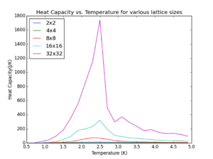
Observations: As predicted by Onsager, the heat capacity spikes for each lattice size around a particular region where the Curie temperature for each lattice is. Overall this is in the region 2.0-2.8K. Furthermore it can be seen that for larger lattice sizes this spike is more pronounced and is accounted for by the fact that the heat capacity for a larger lattice will be higher at it is an extensive property by definition. More importantly this spike occurs at slightly lesser temperatures as lattice size increases. [Note] Heat capacity values plotted are not ‘per spin’ in order to give a realistic value for the entire lattice systems. It is seen that as the lattice size increases the peak in the heat capacity during the phase transition at Tc for the finite lattices is diverging.
Locating the Curie temperature
a) As a validity check for the data obtained through my IsingLattice () model, data is plotted against C++ data obtained from much more extensive cycles. This was done for all lattice sizes, the resulting plot for the 8x8 lattice data set is shown below and the in the appendix for the other lattices.
This utilised a tuple and a figure label list indented in a for loop and plotted 5 subplots per figure, each data file was imported and given and assigned a specific variable to be used in a list. This was in top to bottom order; energy per spin vs. t, energy squared per spin vs. t, magnetisation per spin vs. t, magnetisation squared per spin vs. t and variance per spin vs. t, where t=temperature.
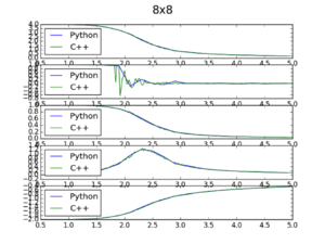
JC: Nice, neat plots. Try to include axis labels on the plots rather than explaining them in the text above.
Observations; It can be seen that the fit of the python data compared to the C++ data is good, but deviates as the Curie temperature for larger lattice sizes. Furthermore the energy squared per spin data from python does not pick up on long-range fluctuations as the system approaches the curie temperature and this is seen for all lattice sizes. Other lattice plots are seen in the appendix. Overall the data fit between the two files is good, leading to confidence in the data obtained via the IsingLattice python function. The code utilised for this is shown below. Furthermore a spike in the variance/fluctuations is shown very clearly in the C++ data especially in the magnetisation vs. temp graphs, with more runs of the MonteCarlo() cycles the Python script would be able to demonstrate this also.
<code>
from IsingLattice import *
from matplotlib import pylab as pl
import numpy as np
a = np.loadtxt("2x2NEW2.dat")
b = np.loadtxt("4x4NEW2.dat")
c = np.loadtxt("8x8NEW2.dat")
d = np.loadtxt("16x16NEW2.dat")
e = np.loadtxt("32x32NEW2.dat")
path_cpp = "../C++_data/"
f = np.loadtxt(path_cpp + "2x2.dat")
g = np.loadtxt(path_cpp + "4x4.dat")
h = np.loadtxt(path_cpp + "8x8.dat")
i = np.loadtxt(path_cpp + "16x16.dat")
j = np.loadtxt(path_cpp + "32x32.dat")
x = [(a, f), (b, g), (c, h), (d, i), (e, j)] #create list of tuples for each combination of python and C++ lattice size datasets
latt_size = ['2x2', '4x4', '8x8', '16x16', '32x32']
for m, (n, o) in enumerate(x):
fig = pl.figure(m + 1)
fig.suptitle(latt_size[m], fontsize=20) #index's the tuple with the latt size list in the for loop
for p in range(5): # p is used enumerate through each of the 5 measures (starting at p+1 since p starts at zero)
pl.subplot(5, 1, p)
pl.plot(n[:, 0], n[:, p + 1])
pl.plot(o[:, 0], o[:, p + 1])
pl.legend(['Python', 'C++'], loc='upper left')
pl.show()
</code>
b) Further analysis is undertaken by fitting the heat capacity vs. t data to a polynomial in order to obtain a functional representation of the graphs via polynomial coefficients. This is firstly done for the whole of the temperature range, via importing the data and indexing the columns appropriately and using np.min/max functions and the np.polyfit(x, y, degree) operator and then unpacking the coefficients using np.polyval to evaluate the coefficients across the entire temperature range; 0.5-5K. The fit was plotted using a np.linspace function to generate 1000 data points in the temperature interval specified. The script is written is a way that uses an‘i’ variable to pick out specific lattice size data. Source code found below.
<code>
from matplotlib import pylab as pl
import numpy as np
a = np.loadtxt("2x2NEW2.dat")
b = np.loadtxt("4x4NEW2.dat")
c = np.loadtxt("8x8NEW2.dat")
d = np.loadtxt("16x16NEW2.dat")
e = np.loadtxt("32x32NEW2.dat")
fig = pl.figure()
i = c #can pick out a specific lattice data set for analysis
T = i[:, 0]
HC = i[:, 5]
fit = np.polyfit(T, HC, 4)#polyfit fits a polynomial a + bx + cx^2 + dx^3 to the data points, saving the coefficients
T_min = np.min(T)
T_max = np.max(T)
T_range = np.linspace(T_min, T_max, num = 1000)
fitted_C_values = np.polyval(fit, T_range)#polyval then evaluates the polynomial values in a data set range T_range- giving a new set of data points
enerax = fig.add_subplot(2, 1, 1)
enerax.set_ylabel("Heat capacity no-fit (J/K)")
enerax.set_xlabel("Temperature (K)")
magax = fig.add_subplot(2, 1, 2)
magax.set_ylabel("Heat capacity fitted (J/K)")
magax.set_xlabel("Temperature (K)")
enerax.plot(T, HC)
magax.plot(T_range ,fitted_C_values)
enerax.legend(['2x2', '4x4', '8x8', '16x16', '32x32'], loc='upper left')
magax.legend(['2x2', '4x4', '8x8', '16x16', '32x32'], loc='upper left')
label = enerax.legend
pl.show()
</code>
JC: Good understanding of the use of polyval and polyfit.
This was done and the optimal polynomial fit was of order 4, as the original data resembles a parabola, however the fit needs increases polynomial order to account for the sharper peak. The result for the 2x2 lattice is shown below.
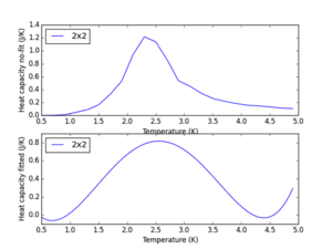
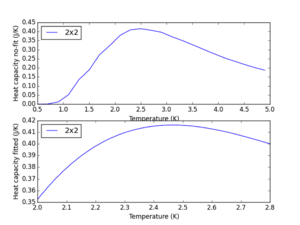
Using a polyfit function for an entire curve is useful, but we are only interested in evaluating the peak region, and therefore limiting it to inside this region, and obtaining the output can optimise the fit. Modifying the code to a selected temperature range, 2.0-2.8k as this is a temperature range where the heat capacity for all systems peaks, for heat capacity data fitting and outputting the fitted heat capacity values only in this region optimises the fit. This is because the polyfit function is not trying to fit polynomial coefficients to the whole temperature range, but only to the one of interest. This is achieved by generating the variables peak_T_range, and fitted_C_values. The source code for this is found below.
<code>
from matplotlib import pylab as pl
import numpy as np
a = np.loadtxt("2x2NEW2.dat")
b = np.loadtxt("4x4NEW2.dat")
c = np.loadtxt("8x8NEW2.dat")
d = np.loadtxt("16x16NEW2.dat")
e = np.loadtxt("32x32NEW2.dat")
fig = pl.figure()
i = a
T = i[:, 0]
HC = i[:, 5]
T_Cmin = 2.0
T_Cmax = 2.8
T_min = np.min(T)
T_max = np.max(T)
selection = np.logical_and(T > T_Cmin, T < T_Cmax) # boolean indexing to select T values in the range Cmin to Cmax
peak_T_values = T[selection]
peak_C_values = HC[selection]
fit = np.polyfit(peak_T_values, peak_C_values, 3)
peak_T_range = np.linspace(T_Cmin, T_Cmax, num = 1000) # linspace creates 1000 data points in temp range chosen to fit polynomial to.
fitted_C_values = np.polyval(fit, peak_T_range)
enerax = fig.add_subplot(2, 1, 1)
enerax.set_ylabel("Heat capacity no-fit (J/K)")
enerax.set_xlabel("Temperature (K)")
magax = fig.add_subplot(2, 1, 2)
magax.set_ylabel("Heat capacity fitted (J/K)")
magax.set_xlabel("Temperature (K)")
enerax.plot(T, HC)
magax.plot(peak_T_range, fitted_C_values)
enerax.legend(['2x2', '4x4', '8x8', '16x16', '32x32'], loc='upper left')
magax.legend(['2x2', '4x4', '8x8', '16x16', '32x32'], loc='upper left')
label = enerax.legend
C_max = np.max(fitted_C_values)
T_max = peak_T_range[fitted_C_values == C_max]
pl.show()
print(C_max, T_max)
</code>
This was done and the optimal polynomial fit was of order 4 for the same reasons as before. The output for the 2x2 lattice is shown below.
JC: Would a higher order polynomial have given a closer fit?
Using the new optimised polynomial peak fits; the maximum heat capacity and its corresponding temperature data points can be abstracted. This is achieved incorporating Cmax = np.max(fitted_C _values) followed by Tmax = peak_T_range[fitted_C_values == Cmax]. This data was outputted and saved in a text file, "python curie temp approx. txt", containing two columns; lattice length l and Tmax. Source code utilised is as used previously in this section, but with the following added functionality to obtain the key data. Text file data shown in table below.
|
2D Ising lattice side length |
Temperature at which C is a max (Tc) |
|
2 |
2.46526527 |
|
4 |
2.38598599 |
|
8 |
2.34434434 |
|
16 |
2.30190190 |
|
32 |
2.19539540 |
<code>
C_max = np.max(fitted_C_values)
T_max = peak_T_range[fitted_C_values == C_max]
print(C_max, T_max)
</code>
Utilising the following scaling relation relating Tc for a finite lattice to Tc for an infinite lattice;

A linear regression script was written in python via importing the txt file data and using code m,b = np.polyfit(x, y, 1), and then outputting b the y-intercept which is equal to . Source code and output line plot below.

JC: Where is the linear regression line in this plot? Joining up the points by straight lines is quite misleading, it would be clearer to just plot your data as points.
<code>
from matplotlib import pylab as pl
import numpy as np
data = np.loadtxt("python curie temp approx.txt")
fig = pl.figure()
Tc = data[:, 1]
Lattlen = 1/(np.array(data[:, 0])) # determination of data sets used in the y = mx + c plot
pl.plot(Lattlen, Tc)
m,b = np.polyfit(Lattlen, Tc, 1)
print(b)
pl.title("Linear regression to determine Tc for an infinite lattice")#dont need A constant as we are only interested in the y-intercept for Tc infinite 2D latt
pl.ylabel("Tc,L (K)")
pl.xlabel("1/L")
pl.show()
</code>
Y-intercept = 2.2463797125K. Lars Onsager’s determined the theoretical Curie temperature for an infinite 2D Ising lattice to be 2.269185314K, the error in this result is +/- 1%. Onsager utilised the following relation [1].

JC: Have you used all system sizes for the linear regression, or just the larger systems?
Error analysis
The error in the result for the theoretical infinite 2D Ising lattice value can be attributed to how the TC data for the finite lattices l= 2, 4, 8, 16, 32 was obtained. Firstly the cut-off point of 4500 Monte Carlo runs may be not be exactly equal to the equilibrating period for all lattice sizes in particular the 32x32 lattice where this period is longest. However the error bars for the data were small so this can only be a small source of error. Secondly intermediate local minima meta-stable states may have formed throughout the runs where the final_data was obtained. This would lead to some of the incorporated data not being fluctuations about the systems equilibrium point. In addition more runs could have been taken when calculating the average data values.
More significant sources of error include using a polynomial fit to the heat capacity data at the phase transition point. For the Ising lattice transitioning between its ferromagnetic and paramagnetic state causes the heat capacity to diverge to infinity and become discontinuous as it peaks at Tc. This is dampened for finite lattices but fitting a polynomial to this as the lattice size increases and converges to infinite behaviour where long-range fluctuations are visible, after 8x8, leads to a bad fit. Finally as it is known that the 2x2 and 4x4 lattice sizes weren’t large enough to lead to reasonable physical results, data values for these sets should be eliminated from the linear regression, as it is seen that they deviate from linearity in the scaling relation. Omitting these sets and running trials for intermediate lattice sizes between 8 and 32 would lead to a better linear fit and therefore data value that was closer to the theoretical value determined via Onsager’s relation. However upon removing the 2x2 and 4x4 data sets, the data deviates from the theoretical value downwards. Upon inspection of the plots of the python vs. C++ data in the appendix, it is seen that the heat capacity per spin values for the 32x32 lattice deviate a lot and this is the source of error. This can be accounted for by the fact that the cut-off despite low error bars, actually is too short. It is known 32x32 lattices at T=2.0K take a very long time to equilibrate on the 100000’s of runs and this was not accounted for in the cut-off. This resulted in a value of 2.012K, a worse approximation for the theoretical value. However it must be noted this is purely due to error in the 16x16 and 32x32 data sets as my plots show these in fact converge to show long-range fluctuations as they should.
References
[1] - R. Albert, and A-L. Barabási, Rev. Mod. Phys. 74 (2002) 4797
Appendix
Accelerating code run speed data (raw)
Slow mag, slow energy
Took 64.217159s
Took 64.27629900000001s
Took 64.19219800000002s
Took 64.670774s
Took 63.92942700000003s
Took 64.19099799999998s
Took 64.314731s
Took 64.12510699999996s
Took 64.09174399999995s
Took 64.20866899999999s
AVERAGE= 64.2217106
Fast mag slow energy(new)
Took 64.06209899999999s
Took 63.507130000000004s
Took 63.52340700000002s
Took 63.70164199999999s
Took 63.567950999999994s
Took 64.03124500000001s
Took 63.29038899999995s
Took 63.80433400000004s
Took 63.47986399999991s
Took 63.54554900000005s
AVERAGE= 63.651361
Slow mag fast energy
Took 2.122013s
Took 2.12318s
Took 2.1139779999999995s
Took 2.128309s
Took 2.1437489999999997s
Took 2.125437999999999s
Took 2.1378489999999992s
Took 2.1242959999999975s
Took 2.121333s
Took 2.123118999999999s
AVERAGE= 2.1263264
Fast mag fast energy
Took 1.1121390000000002s
Took 1.1222689999999997s
Took 1.1211180000000005s
Took 1.1128610000000005s
Took 1.1268589999999996s
Took 1.1132969999999993s
Took 1.1050430000000002s
Took 1.1151069999999998s
Took 1.124898s
Took 1.127703s
AVERAGE= 1.1181294
2x2 &4x4 Cutoff analysis plots
Other C++ vs.↵python data plots


