Talk:Mod:ys5513

NJ: A decent start, but it seems you didn't manage to do the final sections. Some of your plots are a little "busy", and it's hard to discern the data. If you have lots of closely spaced data, it's fine to use a thin line instead of points. Conversely, you sometimes used lines where you really needed points - if you data are quite widely space, you shouldn't just plot lines to join up the dots. Specific comments in the text below.

Liquid Simulations

Introduction to molecular dynamics simulation

TASK: Open the file HO.xls. In it, the velocity-Verlet algorithm is used to model the behaviour of a classical harmonic oscillator. Complete the three columns "ANALYTICAL", "ERROR", and "ENERGY": "ANALYTICAL" should contain the value of the classical solution for the position at time , "ERROR" should contain theabsolute difference between "ANALYTICAL" and the velocity-Verlet solution (i.e. ERROR should always be positive -- make sure you leave the half step rows blank!), and "ENERGY" should contain the total energy of the oscillator for the velocity-Verlet solution. Remember that the position of a classical harmonic oscillator is given by (the values of , , and are worked out for you in the sheet).

Figure 1 on the right shows the result obtained for the Error and total energy

TASK: For the default timestep value, 0.1, estimate the positions of the maxima in the ERROR column as a function of time. Make a plot showing these values as a function of time, and fit an appropriate function to the data. Look at how the energy varies with time.

The maximum error increases linearly with respect to time, as shown in figure 2 below.

TASK: Experiment with different values of the timestep. What sort of a timestep do you need to use to ensure that the total energy does not change by more than 1% over the course of your "simulation"? Why do you think it is important to monitor the total energy of a physical system when modelling its behaviour numerically?

Shorter timespteps lead to more accurate results, but more computing power is needed to simulate the same amount of time. Longer timesteps on the other hand are quicker, but yield less accurate results. Through trial and error it was worked out that a timestep of 0.2 gave an error of 1%. Thus any timestep with this value or shorter should give reasonably accurate results. It is important to monitor the total energy, since in real systems the total energy does not vary with time. Thus the fact the total energy varies with time is a shortcoming of the velocity-Verlet algorithm. However, if the timestep is chosen such that these discrepancies are small, then it may still be assumed that acceptable physical behaviour is modelled

TASK: For a single Lennard-Jones interaction, ,

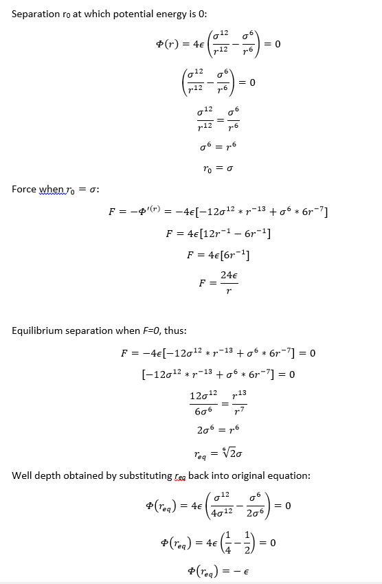
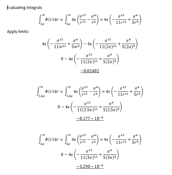
find the separation, , at which the potential energy is zero. What is the force at this separation? Find the equilibrium separation, , and work out the well depth (). Evaluate the integrals , , and when .

NJ: Be careful with these, remember that r is the variable that varies, while sigma is a constant. So the force at a particular location shouldn't depend on r.

TASK: Estimate the number of water molecules in 1ml of water under standard conditions. Estimate the volume of water molecules under standard conditions.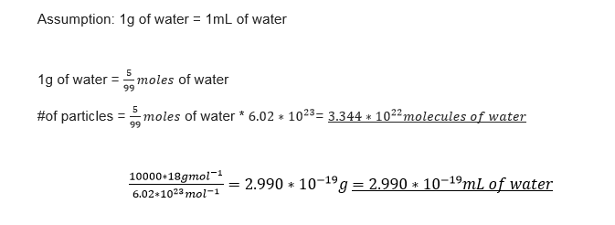

TASK: Consider an atom at position (0.5,0.5,0.5) in a cubic simulation box which runs from(0,0,0) to (1,1,1) . In a single timestep, it moves along the vector (0.7,0.6,0.2). At what point does it end up, after the periodic boundary conditions have been applied?.

Simply moving the particle along the vector would result the new position being (1.3, 1.2, 0.7). However, this is not an acceptable result, since the box is only 1 unit across in all three dimensions. Thus by applying the periodic boundary conditions, it is assumed that if a particle exits the box, then a replica will enter, and will always keep a distance of 1 unit away from the initial particle. Hence the new position of the particle is (0.3, 0.2, 0.7).

NJ: (0.2,0.1,0.7). The initial translation takes the particle to (1.2, 1.1, 0.7).

TASK: The Lennard-Jones parameters for argon are . If the LJ cutoff is , what is it in real units? What is the well depth in ? What is the reduced temperature in real units? 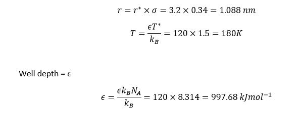NJ: I think you have the units of R wrong. Your answer is 1000 times too big. TASK: Consider again the face-centred cubic lattice from the previous task. How many atoms would be created by the create_atoms command if you had defined that lattice instead?

While a simple cubic lattice has one atom per unit cell, a face centred cubic lattice has 4. Hence the command would create atoms.

NJ: How many?

TASK: Using the LAMMPS manual, find the purpose of the following commands in the input script:

mass 1 1.0: defines mass for all atoms. This in this system only one type of atom is being considered, only one mass needs to be given.

Pair_style lj/cut 3.0: defines which potential governs the interactions between the atoms. In this case the Lennard-Jones potential is applied. Cut 3.0 sets the potential of any atoms apart to 0, as the interaction is considered negligible.

Pari_coeff * * 1.0 1.0: Defines the parameters NJ: Which parameters?

TASK: Given that we are specifying x(0) and v(0) , which integration algorithm are we going to use?

The Velocity Verlet Algorithm.

TASK: Look at the lines below.The second line (starting "variable timestep...") tells LAMMPS that if it encounters the text ${timestep} on a subsequent line, it should replace it by the value given. In this case, the value ${timestep} is always replaced by 0.001. In light of this, what do you think the purpose of these lines is? Why not just write:

This is to ensure that all simulations take place over the same amount of time, such that the results may be compared, and in decreasing the timestep, the number of steps over which the simulation is run increases accordingly. In the latter example, doubling the timestep would also double the amount of time simulated, but with the same degree of accuracy.

TASK: make plots of the energy, temperature, and pressure, against time for the 0.001 timestep experiment (attach a picture to your report). Does the simulation reach equilibrium? How long does this take? When you have done this, make a single plot which shows the energy versus time for all of the timesteps (again, attach a picture to your report). Choosing a timestep is a balancing act: the shorter the timestep, the more accurately the results of your simulation will reflect the physical reality; short timesteps, however, mean that the same number of simulation steps cover a shorter amount of actual time, and this is very unhelpful if the process you want to study requires observation over a long time. Of the five timesteps that you used, which is the largest to give acceptable results? Which one of the five is a particularly bad choice? Why?

The timestep 0.15 gives particularly bad results, since the energy never equilibrates, but rather steadily increases. As the timestep is decreases, the average energy decreases as well. However, qualitatively the timesteps 0.001 and 0.0025 give very similar results. Thus the extra computing power used when the timestep is 0.001 vs. 0.0025 is redundant, and the timestep 0.0025 may be chosen as an optimum value.

N.B. Although the optimum value was chosen to be 0.0025, some of the following calculations inadvertently were run at a timestep of 0.0075. While these result are clearly less accurate, they should still yield results comparable and with similar trends to those run with a timestep of 0.0025. Thus due to time constraints these results will be used.

Running Simulations under specific conditions

TASK: Use the manual page to find out the importance of the three numbers 100 1000 100000. How often will values of the temperature, etc., be sampled for the average? How many measurements contribute to the average? Looking to the following line, how much time will you simulate?

100 (Nevery): for each average calculation values will be selected as follows: x-100, x-200, x-300 such that this occurs Nrepeat(=1000) number of times, where x is equal to or a multiple of Nfreq.

1000(Nrepeat): how many values of timesteps are used for each average calculation

100000(Nfreq): a new average will be calculated in intervals of this many timesteps

TASK: When your simulations have finished, download the log files as before. At the end of the log file, LAMMPS will output the values and errors for the pressure, temperature, and density . Use software of your choice to plot the density as a function of temperature for both of the pressures that you simulated. Your graph(s) should include error bars in both the x and y directions. You should also include a line corresponding to the density predicted by the ideal gas law at that pressure. Is your simulated density lower or higher? Justify this. Does the discrepancy increase or decrease with pressure?

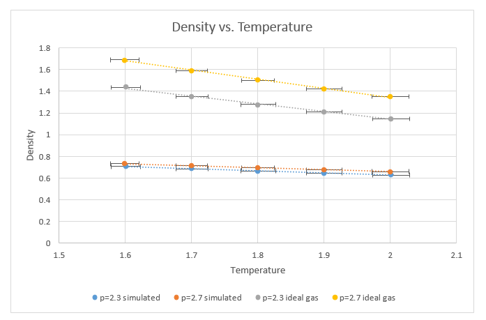
The graph above shows the densities plotted as a function of temperature at 2 different pressures. The densities used were obtained using the LAMMPS software in one case and using the ideal gas law in the other case. Vertical error bars are present, but the error is too small to be depicted. In addition

Density increases with increasing pressure and decreases with increasing temperature, as would be expected. The densities calculated using the ideal gas law are considerably greater. This is as a result of the ideal gas law not taking into account any interaction between particles. This would also explain why increasing the pressure increases the density of the “ideal gas” density more than it does the “Lennard Jones” density, since packing the “Lennard Jones” particles too tightly results in strong repulsive forces counteracting the effects of the pressure.

However, extrapolating these lines forward would result in the discrepancies between these models to decrease, since at higher temperatures (and thus higher higher kinetic energy) intermolecular interaction become less significant. Similarly, the discrepancy increases with increasing pressure, also do to the potential between the atoms in the Lennard-Jones model, which is neglected in the ideal gas model.

Calculating heat capacities using statistical physics

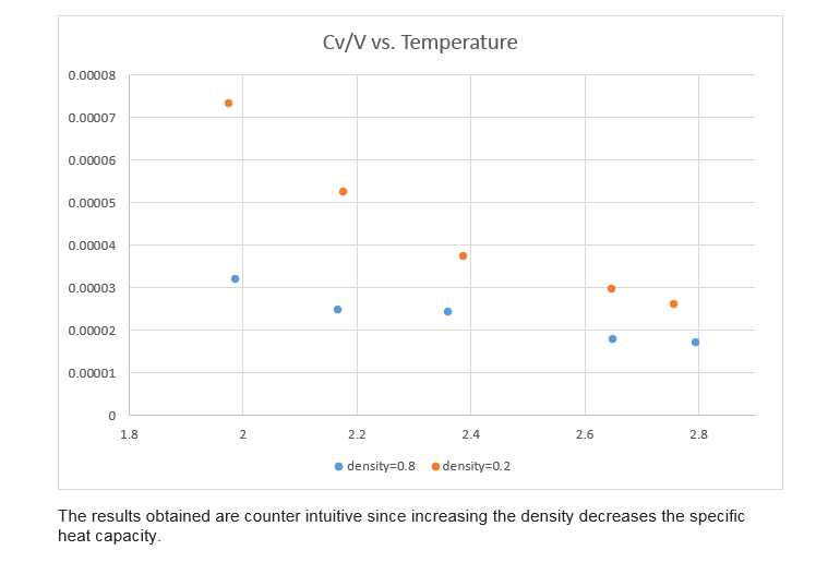
TASK: As in the last section, you need to run simulations at ten phase points. In this section, we will be in density-temperature phase space, rather than pressure-temperature phase space. The two densities required at and , and the temperature range is . Plot as a function of temperature, where is the volume of the simulation cell, for both of your densities (on the same graph). Is the trend the one you would expect? Attach an example of one of your input scripts to your report.

The script used for the calculations is depicted below:

### DEFINE SIMULATION BOX GEOMETRY ###

lattice sc 0.8

region box block 0 15 0 15 0 15

create_box 1 box

create_atoms 1 box

### DEFINE PHYSICAL PROPERTIES OF ATOMS ###

mass 1 1.0

pair_style lj/cut/opt 3.0

pair_coeff 1 1 1.0 1.0

neighbor 2.0 bin

### SPECIFY THE REQUIRED THERMODYNAMIC STATE ###

variable T equal ...

variable timestep equal 0.0025

### ASSIGN ATOMIC VELOCITIES ###

velocity all create ${T} 12345 dist gaussian rot yes mom yes

### SPECIFY ENSEMBLE ###

timestep ${timestep}

fix nve all nve

### THERMODYNAMIC OUTPUT CONTROL ###

thermo_style custom time etotal temp press

thermo 10

### RECORD TRAJECTORY ###

dump traj all custom 1000 output-1 id x y z

### SPECIFY TIMESTEP ###

### RUN SIMULATION TO MELT CRYSTAL ###

run 10000

unfix nve

reset_timestep 0

### BRING SYSTEM TO REQUIRED STATE ###

variable tdamp equal ${timestep}*100

variable pdamp equal ${timestep}*1000

fix nvt all nvt temp ${T} ${T} ${tdamp}

run 10000

unfix nvt

fix nve all nve

reset_timestep 0

### MEASURE SYSTEM STATE ###

thermo_style custom step etotal temp press density atoms vol

variable vol equal vol

variable dens equal density

variable dens2 equal density*density

variable temp equal temp

variable temp2 equal temp*temp

variable press equal press

variable press2 equal press*press

variable energy1 equal etotal*etotal

variable energy2 equal etotal

variable atoms equal atoms

fix aves all ave/time 100 1000 100000 v_dens v_temp v_press v_dens2 v_temp2 v_press2 v_energy1 v_energy2

run 100000

variable avedens equal f_aves[1]

variable avetemp equal f_aves[2]

variable avepress equal f_aves[3]

variable errdens equal sqrt(f_aves[4]-f_aves[1]*f_aves[1])

variable errtemp equal sqrt(f_aves[5]-f_aves[2]*f_aves[2])

variable errpress equal sqrt(f_aves[6]-f_aves[3]*f_aves[3])

variable htcpcty equal ((atoms)*(atoms)*(f_aves[7]-(f_aves[8]*f_aves[8])))/f_aves[5]

print "Averages"

NJ: What about the density dependence? This isn't the specific heat capacity, by the way - it's not per mole.

Structural Properties and the radial distribution function

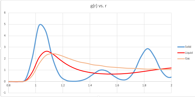
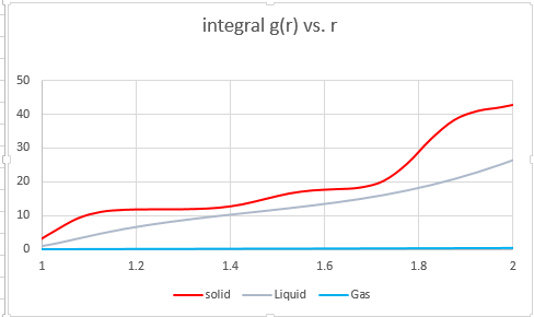
The nature of these peaks sheds light on how much order is present in all three phases. The solid phase is highly ordered, and thus the nearest neighbour as well as the voids may be predicted with reasonable accuracy. In a perfect solid structure at a very low temperature, the nature of the curve would be even more sinusoidal, but due to thermal motion and imperfections in the crystal lattice, there are deviations.

NJ: Do you mean it would be a delta function?

The liquid phase has far less order, certainly at long range. Yet there is short range order (solvent shells), but then the peaks quickly flatten out and become equal to the density. The gas phase predictably is the least ordered, and while the nearest neighbours may also be predicted with a reasonable degree of accuracy, beyond that there is no well defined order.