Talk:Mod:wkl13

JC: General comments: All tasks completed with a few mistakes. Make sure that you understand the background theory behind the tasks so that you understand what your results show.

Introduction

Task 1

Open the file HO.xls. In it, the velocity-Verlet algorithm is used to model the behaviour of a classical harmonic oscillator. Complete the three columns "ANALYTICAL", "ERROR", and "ENERGY": "ANALYTICAL" should contain the value of the classical solution for the position at time $t$, "ERROR" should contain the absolute difference between "ANALYTICAL" and the velocity-Verlet solution (i.e. ERROR should always be positive -- make sure you leave the half step rows blank!), and "ENERGY" should contain the total energy of the oscillator for the velocity-Verlet solution. Remember that the position of a classical harmonic oscillator is given by $x\left(t\right)=A\cos (\omega t+\varphi )$ (the values of $A$, $\omega$, and $\varphi$ are worked out for you in the sheet).

For a classical harmonic oscillator, each particles will experience a force. The analytical position x(t) can be described by the function

$x\left(t\right)=A\cos (\omega t+\varphi )$

The error is the absolute of the differences between the Verlet algorithm and the analytical x. The graph below is error plotted against time.

The total energy is the sum of the kinetic and potential energy.

$E(x)=\frac{1}{2}m{v}^2+\frac{1}{2}k{x}^2$

For timestep 0.1,

• 
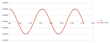  analytical x(t) against time graph
• Energy against time graph
  Energy against time graph
• Error against time graph
  Error against time graph

The total energy is almost constant. Analytically, it should be constant as energy is always conserved. Since the algorithm approach is used, there are sips in between, hence leading the energy fluctuates slightly.

Task 2

For the default timestep value, 0.1, estimate the positions of the maxima in the ERROR column as a function of time. Make a plot showing these values as a function of time, and fit an appropriate function to the data.

local maxima	1st	2nd	3rd	4th	5th
positions	7.58E-04	2.01E-03	3.30E-03	4.60E-03	5.91E-03
time	2.0	4.9	8.0	11.1	14.2

Error plot max against time

Error plot max against time

A positive linear correlation is found. All the points satisfy into y =0.004x-0.00007 with $R^2=1$.

JC: Is the fit really perfect (R^2 = 1)? Give the line of best fit and R^2 value to more than 1 significant figure.

Task 3

Experiment with different values of the timestep. What sort of a timestep do you need to use to ensure that the total energy does not change by more than 1% over the course of your "simulation"? Why do you think it is important to monitor the total energy of a physical system when modelling its behaviour numerically?

Different values of timestep have been used to explore the percentage of change in total energy. It is found $x<0.2$ does not change the total energy by more than 1%. Analytically, by the conservation of energy, energy is always conserved. However, in the algorithm approach, the Taylor expansion only expands to the power of 3, in which the calculated value is not exact, hence there is a difference in energy. 1% is the benchmark.

JC: Good choice of timestep, but which other timesteps did you try?

Task 4

For a single Lennard-Jones interaction, $\varphi \left(r\right)=4ϵ(\frac{{\sigma }^{12}}{r^{12}}-\frac{{\sigma }^6}{r^6})$, find the separation, $r_0$, at which the potential energy is zero. What is the force at this separation? Find the equilibrium separation, $r_{eq}$, and work out the well depth ($\varphi \left(r_{eq}\right)$). Evaluate the integrals $\underset{2\sigma }{\overset{\mathrm{\infty }}{\int }}\varphi \left(r\right)\mathrm{d}r$, $\underset{2.5\sigma }{\overset{\mathrm{\infty }}{\int }}\varphi \left(r\right)\mathrm{d}r$, and $\underset{3\sigma }{\overset{\mathrm{\infty }}{\int }}\varphi \left(r\right)\mathrm{d}r$ when $\sigma =ϵ=1.0$.

The potential energy is given by the Lennard-Jones equation

$\varphi \left(r\right)=4ϵ(\frac{{\sigma }^{12}}{r^{12}}-\frac{{\sigma }^6}{r^6})$

when $\varphi \left(r\right)=0$,

$4ϵ(\frac{{\sigma }^{12}}{r_0^{12}}-\frac{{\sigma }^6}{r_0^6})=0$

$\frac{{\sigma }^{12}}{r_0^{12}}=\frac{{\sigma }^6}{r_0^6}$

$r_0^6={\sigma }^6$

$r_0=\sigma$

For a single interaction,

${\mathbf{F}}_i=-\frac{\mathrm{d}U\left({\mathbf{r}}^N\right)}{\mathrm{d}{\mathbf{r}}_i}$

Consider the Lennard-Jones interaction is the only source of potential energy,

${\mathbf{F}}_i=-\frac{\mathrm{d}4ϵ(\frac{{\sigma }^{12}}{r^{12}}-\frac{{\sigma }^6}{r^6})}{\mathrm{d}{\mathbf{r}}_i}$

$=-4ϵ(\frac{-12{\sigma }^{12}}{r^{13}}+6\frac{{\sigma }^6}{r^7})$

$=48ϵ\frac{{\sigma }^{12}}{r^{13}}-24ϵ\frac{{\sigma }^6}{r^7}$

for $r=\sigma$,

$\mathbf{F}=48ϵ\frac{{\sigma }^{12}}{{\sigma }^{13}}-24ϵ\frac{{\sigma }^6}{{\sigma }^7}$

$=48\frac{ϵ}{\sigma }-24\frac{ϵ}{\sigma }$

$=24\frac{ϵ}{\sigma }$

At equilibrium $r_{eqm}$, the potential energy reaches the minimum, hence $\frac{\mathrm{d}U}{\mathrm{d}r}=0$.

$\frac{\mathrm{d}U}{\mathrm{d}r}=-4ϵ(\frac{-12{\sigma }^{12}}{r_{eqm}^{13}}+6\frac{{\sigma }^6}{r_{eqm}^7})=0$

$\frac{-12{\sigma }^{12}}{r_{eqm}^{13}}+6\frac{{\sigma }^6}{r_{eqm}^7}=0$

$\frac{12{\sigma }^{12}}{r_{eqm}^{13}}=\frac{6{\sigma }^6}{r_{eqm}^7}$

$2{\sigma }^6=r_{eqm}^6$

$r_{eqm}=2^{1/6}\sigma$

Well depth $\varphi \left(r_{eqm}\right)=\varphi \left(2^{1/6}\sigma \right)$

$=4ϵ(\frac{{\sigma }^{12}}{(\sigma (2{)}^{1/6}{)}^{12}}-\frac{{\sigma }^6}{(\sigma (2{)}^{1/6}{)}^6})$

$=4ϵ(\frac{1}{2^2}-\frac{1}{2})$

$=-ϵ$

$\underset{2\sigma }{\overset{\mathrm{\infty }}{\int }}\varphi \left(r\right)\mathrm{d}r$

$=\underset{2\sigma }{\overset{\mathrm{\infty }}{\int }}4ϵ(\frac{{\sigma }^{12}}{r^{12}}-\frac{{\sigma }^6}{r^6})\mathrm{d}r$

$=4ϵ({\sigma }^{12}\underset{2\sigma }{\overset{\mathrm{\infty }}{\int }}\frac{1}{r^{12}}\mathrm{d}r-{\sigma }^6\underset{2\sigma }{\overset{\mathrm{\infty }}{\int }}\frac{1}{r^6}\mathrm{d}r)$

$=-0.248$

Similarly,

$\underset{2.5\sigma }{\overset{\mathrm{\infty }}{\int }}\varphi \left(r\right)\mathrm{d}r=-0.00818$

$\underset{3\sigma }{\overset{\mathrm{\infty }}{\int }}\varphi \left(r\right)\mathrm{d}r=-0.00329$

Task 5

Estimate the number of water molecules in 1ml of water under standard conditions. Estimate the volume of $10000$ water molecules under standard conditions.

Under standard conditions [101 kPa, 298K] ,

$\text{density of water}=0.997gm{l}^{-1}$

$Mr\left(water\right)=18.02gmo{l}^{-1}$

$\text{no. of moles}=\frac{mass}{Mr}=\frac{\text{no. of molecules}}{\text{Avogadro's constant}}$

$\text{no. of water molecules}=\frac{mass}{Mr}\times 6.02\times 10^{23}$

$=\frac{0.997}{18.02}\times 6.02\times 10^{23}$

$=3.34\times 10^{22}$

$\text{mass of water}=\frac{\text{no. of molecules}}{\text{Avogadro's constant}}\times Mr$

$=\frac{10000}{6.02\times 10^{23}}\times 18.02$

= 2.99 x 10^{-19} g

$\text{Volume}=\frac{mass}{density}$

$=\frac{2.99\times 10^{-19}}{0.997}$

= 3.00 x 10^{-19} cm^{3}

JC: All maths and calculations correct and nicely laid out.

Task 6

Consider an atom at position $(0.5,0.5,0.5)$ in a cubic simulation box which runs from $(0,0,0)$ to $(1,1,1)$. In a single timestep, it moves along the vector $(0.7,0.6,0.2)$. At what point does it end up, after the periodic boundary conditions have been applied?

$(0.5,0.5,0.5)+(0.7,0.6,0.2)$

$=(1.2,1.1,0.7)$

(Using periodic boundary condition*)

$=(0.2,0.1,0.7)$

• Periodic boundary condition: if particle moves out of the box $(1,1,1)$, the box will move back and particle will appear in the box again.

JC: Values correct, but use the same number of significant figures as are given in the question (in this case 2).

Task 7

The Lennard-Jones parameters for argon are $$\begin{gathered} \sigma =0.34\mathrm{n}\mathrm{m},ϵ \\ / \\ {k}_B=120\mathrm{K} \end{gathered}$$. If the LJ cutoff is $r^{*}=3.2$, what is it in real units? What is the well depth in $$\begin{gathered} {\mathrm{k}\mathrm{J} \\ \mathrm{m}\mathrm{o}\mathrm{l}}^{-1} \end{gathered}$$? What is the reduced temperature $T^{*}=1.5$ in real units?

$r=\frac{r^{*}}{\sigma }$

$=3.2\times 0.34\mathrm{n}\mathrm{m}$

$=1.09\mathrm{n}\mathrm{m}$

$\text{Well Depth}=4ϵ(\frac{{\sigma }^{12}}{r^{12}}-\frac{{\sigma }^6}{r^6})$

$$\begin{gathered} =4\times 120 \\ {k}_B\times (3.2^{-12}-3.2^{-6}) \end{gathered}$$

$=-6.17\times 10^{-24}\mathrm{k}\mathrm{J}\mathrm{m}\mathrm{o}{\mathrm{l}}^{\mathrm{-}\mathrm{1}}$

$T^{*}=\frac{k_{B}T}{ϵ}$

$T=\frac{T^{*}ϵ}{k_B}$

$=1.5\times 120\mathrm{K}$

$=180\mathrm{K}$

Equilibration

Task 1

Why do you think giving atoms random starting coordinates causes problems in simulations? Hint: what happens if two atoms happen to be generated close together?

Atoms with random starting coordinates have a chance of superposing each other, which is impractical in reality. No two atoms can rest on the same space.

When two atoms are too close (the separation distance is small), according to the Lennard-Jones Potential, the potential energy is very high, as the atoms are repulsing each other. Therefore, the simulation does not fit into real case.

JC: What do you mean by "does not fit into a real case"? The problem with a simulation with high repulsion is that the simulation will be unstable and a smaller timestep will be needed to stop it from crashing.

Task 2

Satisfy yourself that this lattice spacing corresponds to a number density of lattice points of $0.8$. Consider instead a face-centred cubic lattice with a lattice point number density of 1.2. What is the side length of the cubic unit cell?

$\text{number density}=\frac{\text{no of atoms}}{\text{volume}}$

$\text{volume}={\text{length}}^3$

For a simple cubic lattice,

$\text{no of atoms}=8\times \frac{1}{8}=1$

$\text{number density}=\frac{1}{1.07722^3}=0.800(3s.f.)$

For a face-centred cubic lattice,

$\text{no of atoms}=8\times \frac{1}{8}+6\times \frac{1}{2}=1+3=4$

$\text{volume}={\text{length}}^3=\frac{\text{no of atoms}}{\text{number density}}=\frac{4}{1.2}$

${\text{length}}^3=3.\dot{3}$

$\text{length}=1.49\left(\text{in reduced units}\right)$

Task 3

Consider again the face-centred cubic lattice from the previous task. How many atoms would be created by the create_atoms command if you had defined that lattice instead?

$\text{no of atoms per FCC lattice}=4$

1 box creates 1000 unit cells

$\text{no of atoms created}=4\times 1000=4000$

JC: Correct.

Task 4

Using the LAMMPS manual , find the purpose of the following commands in the input script:

mass 1 1.0
pair_style lj/cut 3.0
pair_coeff * * 1.0 1.0

mass 1 1.0	This is a mass command. '1' refers to the atom type while '1.0' refers to the mass value.
pair_style lj/cut 3.0	This command implies only considering the Lennard-Jones potential up to 3.0 atomic units.
pair_coeff * * 1.0 1.0	This is a pair coefficient command. The asterick (*) with no values refer all types of atom from 1 to N. The 1.0 1.0 refers to the atom type '1.0' interacting with '1.0'.

JC: Why is a cutoff used for the Lennard-Jones potential? In the pair_coeff command, the "1.0"s correspond to the values for sigma and epsilon.

Task 5

Given that we are specifying ${\mathbf{x}}_i\left(0\right)$ and ${\mathbf{v}}_i\left(0\right)$, which integration algorithm are we going to use?

Velocity-Verlet algorithm ${\mathbf{v}}_i\left(0\right)$

For classical Verlet algorithm ${\mathbf{x}}_i\left(0\right)$,the initial conditions only require ${\mathbf{x}}_i\left(0\right)$ and ${\mathbf{x}}_i(-\delta t)$;

while velocity Verlet algorithm ${\mathbf{v}}_i\left(0\right)$ require ${\mathbf{x}}_i\left(0\right)$ and ${\mathbf{v}}_i\left(0\right)$ only.

JC: Good understanding.

Task 6

Look at the lines below.

### SPECIFY TIMESTEP ###
variable timestep equal 0.001
variable n_steps equal floor(100/${timestep})
variable n_steps equal floor(100/0.001)
timestep ${timestep}
timestep 0.001

### RUN SIMULATION ###
run ${n_steps}
run 100000

The second line (starting "variable timestep...") tells LAMMPS that if it encounters the text ${timestep} on a subsequent line, it should replace it by the value given. In this case, the value ${timestep} is always replaced by 0.001. In light of this, what do you think the purpose of these lines is? Why not just write:

timestep 0.001
run 100000

The timestep command fixes the time interval for each run. The advantage of using the lines in the top box is flexibility. When the timestep is varied in the future experiment, the run will change automatically, and does not require manual input which could avoid human errors when running the LAMMPS simulation.

JC: Correct.

Task 7

make plots of the energy, temperature, and pressure, against time for the 0.001 timestep experiment (attach a picture to your report). Does the simulation reach equilibrium? How long does this take? When you have done this, make a single plot which shows the energy versus time for all of the timesteps (again, attach a picture to your report). Choosing a timestep is a balancing act: the shorter the timestep, the more accurately the results of your simulation will reflect the physical reality; short timesteps, however, mean that the same number of simulation steps cover a shorter amount of actual time, and this is very unhelpful if the process you want to study requires observation over a long time. Of the five timesteps that you used, which is the largest to give acceptable results? Which one of the five is a particularly bad choice? Why?

For timestep = 0.001

• File:Energty against time graph.tif
• File:Temperature against time.tif
• File:Pressure agasint time.tif

The simulation reaches equilibrium, as the energy is almost constant. The fluctuation can be explained by the algorithm used, which only approximates up to the third term of Taylor expansion. Equilibrium is reached after 0.3 time units.

A plot of energy against time with different timesteps is shown below:

Energy against time for various timestep

Energy against time for various timestep

Timestep of 0.015 does not reach equilibrium, as the energy is increasing.It is a "particularly" bad choice. Theoretically, by conservation of energy, the total energy should be a constant, which does not depend on the timestep. The timestep we choose for the experiment should give out the same energy. Among the other simulations, timestep of 0.0025 and 0.001 gives similar energies, which indicates the Verlet-algorithm gives a good approximation in these cases. In addition, in running the simulations,we always aim at longer observation time, which could go for longer time. Therefore, timestep of 0.0025 is the largest to give a result which looks like independent of the time.

JC: Good choice and justification of the timestep chosen.

Running simulations under specific conditions

Task 1

Choose 5 temperatures (above the critical temperature $T^{*}=1.5$), and two pressures (you can get a good idea of what a reasonable pressure is in Lennard-Jones units by looking at the average pressure of your simulations from the last section). This gives ten phase points — five temperatures at each pressure. Create 10 copies of npt.in, and modify each to run a simulation at one of your chosen $(p,T)$ points. You should be able to use the results of the previous section to choose a timestep. Submit these ten jobs to the HPC portal. While you wait for them to finish, you should read the next section.

$T^{*}=1.6,1.8,2.0,2.2,2.4$ and $p^{*}=2.0,3.0$ (fluctuate within this range as shown in previous part) were chosen. As explained in previous section, timestep of $0.0025$ was chosen.

Task 2

We need to choose $\gamma$ so that the temperature is correct $T=\mathfrak{𝔗}$ if we multiply every velocity $\gamma$. We can write two equations:

$\frac{1}{2}\sum _i{m}_i{v}_i^2=\frac{3}{2}N{k}_{B}T$

$\frac{1}{2}\sum _i{m}_i{\left(\gamma v_i\right)}^2=\frac{3}{2}N{k}_B\mathfrak{𝔗}$

Solve these to determine $\gamma$.

$\frac{1}{2}\sum _i{m}_i{v}_i^2=\frac{3}{2}N{k}_{B}T\left(1\right)$

$\frac{1}{2}\sum _i{m}_i{\left(\gamma v_i\right)}^2=\frac{3}{2}N{k}_B\mathfrak{𝔗}\left(2\right)$

$\frac{(1)}{(2)}\text{:}\frac{\frac{1}{2}\sum _i{m}_i{v}_i^2}{\frac{1}{2}\sum _i{m}_i{\left(\gamma v_i\right)}^2}=\frac{\frac{3}{2}N{k}_{B}T}{\frac{3}{2}N{k}_B\mathfrak{𝔗}}$

$\frac{1}{{\gamma }^2}=\frac{T}{\mathfrak{𝔗}}$

${\gamma }^2=\frac{\mathfrak{𝔗}}{T}$

$\gamma =\sqrt{\frac{\mathfrak{𝔗}}{T}}$

JC: Clear derivation.

Task 3

fix aves all ave/time 100 1000 100000 v_dens v_temp v_press v_dens2 v_temp2 v_press2
run 100000

Use the Manual pageto find out the importance of the three numbers 100 1000 100000. How often will values of the temperature, etc., be sampled for the average? How many measurements contribute to the average? Looking to the following line, how much time will you simulate?

The lines indicate:

100	Nevery, refers to the use values every 100 timesteps.
1000	Nrepeat, refers to the number of times to use the input values for calculating the averages.
100000	Nfreq, calculates the averages every 100000 timesteps.

The values of the temperature is recorded every 100 step.

The values are sampled every 100000 timesteps.

1000 measurements contribute to the average.

1000000 will be used to complete the simulation.

JC: What do you mean by "values are sampled every 100000 timesteps"? The average is calculated every 100000 steps.

Task 4

When your simulations have finished, download the log files as before. At the end of the log file, LAMMPS will output the values and errors for the pressure, temperature, and density $\left(\frac{N}{V}\right)$. Use software of your choice to plot the density as a function of temperature for both of the pressures that you simulated. Your graph(s) should include error bars in both the x and y directions. You should also include a line corresponding to the density predicted by the ideal gas law at that pressure. Is your simulated density lower or higher? Justify this. Does the discrepancy increase or decrease with pressure?

The ideal gas model can also be used to approximate the gases, which assumes

(1) negligible intermolecular forces between the gas molecules

(2) perfectly elastic collisions between the molecule and with the container walls is the only interactions

(3) negligible volume occupied by the molecules compared to container

It can be described mathematically as shown below

$pV=nRT$

where p is pressure, V is the volume, n is number of moles, R is the gas constant and T is temperature.

Since $nR=N{k}_B$, where N is the number of atoms and $k_B$ is the Boltzmann's constant.

$k_B=1(\text{in reduced units})$

$pV=NT$

$\frac{N}{V}=\frac{p}{T}$

$\text{density}\rho =\frac{p}{T}$

Apart from running simulation, density can also be calculated from the the ideal gas law by dividing pressure by temperature.

The error bars are based on standard deviations $\sigma$ from the simulation, while $\sigma \left(\rho \right)$ was calculated using the following equation

$\sigma \left(\rho \right)=\sqrt{{\left(\frac{\sigma \left(p\right)}{p}\right)}^2+{\left(\frac{\sigma \left(T\right)}{T}\right)}^2}$

JC: The standard error should be printed out by at the end of the simulation. Using density = pressure/temperature to calculate the error is not necessarily valid for the simulations as it assumes the ideal gas law applies to the simulations.

Assuming positive and negative error bar is the same in magnitude. The error bar stimulated density are too small (~$10^{-2}$)to be shown on the graph.

Here is the plot of density as a function of temperature in two different (controlled) pressure, under simulation and ideal gas approximation.

Density against temp revised

Density against temp revised

The simulated density is lower than the calculated. This phenomenon can be explained by the assumption of gas molecules do not interact with each other in the ideal gas approximation model. In a fixed volume, more gas molecules can be found as the molecules do not repel with each other, hence density is higher.

The plot shows

(1)Density is inversely proportional to temperature. Negative gradients were found in the density against temperature graph.

When temperature increases, the average kinetic energy increases, molecules are more energetic, and moving at a higher speed. In a fixed volume, fewer molecules are found (i.e. density decreases).

(2)Discrepancy in density increases, as pressure increases. Densities were observed to be higher at $p^{*}=3.0$than $p^{*}=2.0$(while other variables kept constant). The discrepancy between the simulation and the ideal gas model (i.e. less exact) increases when $p^{*}$ increases from 2.0 to 3.0.

When pressure increases, molecules are forced closer together and interact stronger. Consequently, volume at a given temperature is decreased, as the number of atoms N is fixed in the simulation ($pV=NT=const$). Density ($\rho =\frac{N}{V}$)at the given temperature increases, as the volume decreases. There will be more interaction between molecules which has been neglected in the ideal gas assumption. Hence, the ideal gas model breaks down, larger discrepancy will be observed.

JC: Good explanations. What happens to the discrepancy between the ideal gas and the simulation results as temperature increases?

Calculating heat capacities using statistical physics

Task 1

As in the last section, you need to run simulations at ten phase points. In this section, we will be in density-temperature $({\rho }^{*},T^{*})$ phase space, rather than pressure-temperature phase space. The two densities required at $0.2$ and $0.8$, and the temperature range is $2.0,2.2,2.4,2.6,2.8$. Plot $C_V/V$ as a function of temperature, where $V$ is the volume of the simulation cell, for both of your densities (on the same graph). Is the trend the one you would expect? Attach an example of one of your input scripts to your report.

Input script for ${\rho }^{*}=0.2$ and $T^{*}=2.0$,

### DEFINE SIMULATION BOX GEOMETRY ###
lattice sc 0.2
region box block 0 15 0 15 0 15
create_box 1 box
create_atoms 1 box

### DEFINE PHYSICAL PROPERTIES OF ATOMS ###
mass 1 1.0
pair_style lj/cut/opt 3.0
pair_coeff 1 1 1.0 1.0
neighbor 2.0 bin

### SPECIFY THE REQUIRED THERMODYNAMIC STATE ###
variable T equal 2.0
variable timestep equal 0.0025

### ASSIGN ATOMIC VELOCITIES ###
velocity all create ${T} 12345 dist gaussian rot yes mom yes

### SPECIFY ENSEMBLE ###
timestep ${timestep}
fix nve all nve

### THERMODYNAMIC OUTPUT CONTROL ###
thermo_style custom time etotal temp press
thermo 10

### RECORD TRAJECTORY ###
dump traj all custom 1000 output-1 id x y z

### SPECIFY TIMESTEP ###

### RUN SIMULATION TO MELT CRYSTAL ###
run 10000
unfix nve
reset_timestep 0

### BRING SYSTEM TO REQUIRED STATE ###
variable tdamp equal ${timestep}*100
variable pdamp equal ${timestep}*1000
fix nvt all nvt temp ${T} ${T} ${tdamp} 
run 10000
reset_timestep 0

### MEASURE SYSTEM STATE ###
unfix nvt
fix nve all nve
thermo_style custom step etotal temp press density atoms vol
variable dens equal density
variable dens2 equal density*density
variable temp equal temp
variable temp2 equal temp*temp
variable press equal press
variable press2 equal press*press
variable N equal atoms
variable N2 equal atoms*atoms
variable etotal equal etotal
variable etotal2 equal etotal*etotal
variable volume equal vol
fix aves all ave/time 100 1000 100000 v_dens v_temp v_press v_etotal v_dens2 v_temp2 v_press2 v_etotal2
run 100000

variable avedens equal f_aves[1]
variable avetemp equal f_aves[2]
variable avepress equal f_aves[3]
variable aveetotal equal f_aves[4]
variable aveetotal2 equal f_aves[8]
variable heatcapacity equal ${N2}*(${aveetotal2}-${aveetotal}*${aveetotal})/(${avetemp}*${avetemp})

print "Averages"
print "--------"
print "Density: ${avedens}"
print "Temperature: ${avetemp}"
print "Pressure: ${avepress}"
print "total energy: ${aveetotal}"
print "total energy^2: ${aveetotal2}"
print "heat capacity: ${heatcapacity}"
print "number of atoms: ${N2}"
print "Volume: ${volume}"

Heatcappervolagainsttemp_modified

Heatcappervolagainsttemp_modified

The heat capacity at constant volume per unit volume against time plot is shown above.

The internal energy $U$ varies with temperature and volume.

Heat capacity at constant volume $C_v$ is defined as heat energy per unit temperature.

$C_V=\frac{\partial E}{\partial T}$

The volume is fixed, and we are interested in variation with the temperature. Since heat capacity is proportional to volume, we normalise the system to which is invariant with the size for comparison

Higher $\frac{C_V}{V}$ at specific temperature was observed in ${\rho }^{*}=0.8$ than ${\rho }^{*}=0.2$.

This can be explained molecules are closer at higher density. Higher potential energy is experienced as resulted from stronger interaction between molecules. Hence, the internal energy increases, consequently the thermal energy. Eventually, the $C_V$ increases.

Another observation which out of expectation was also found.

File:Shottky Anomaly.png

Schottky Anomaly

Lower $\frac{C_V}{V}$, as temperature increases.

According to the Schottky anomaly , which the ensemble in simulation is also NVT, at low temperature, there are more vacancies in higher energy states. Molecules are more likely to be populated from lower energy states to higher energy states. Hence, heat capacity is expected to increase.

All simulations were run at high temperatures, (above $T*=2.0=2\times 120K=240K$), therefore no quantum effect can be observed.

JC: Cv/V is higher at higher densities since more molecules are present in a given volume so more energy is required to raise the temperature of the system. Good attempt to explain the trend with temperature, but do you think the Schottky anomaly explains this trend? The simulation is completely classical, so quantum effects are not included in the simulation.

Structural properties and the radial distribution function

Task 1

perform simulations of the Lennard-Jones system in the three phases. When each is complete, download the trajectory and calculate $g(r)$ and $\int g(r)\mathrm{d}r$. Plot the RDFs for the three systems on the same axes, and attach a copy to your report. Discuss qualitatively the differences between the three RDFs, and what this tells you about the structure of the system in each phase. In the solid case, illustrate which lattice sites the first three peaks correspond to. What is the lattice spacing? What is the coordination number for each of the first three peaks?

The simulations were run under these conditions,

solid $\rho =1.2,T*=0.8,\text{fcc}$; liquid $\rho =0.8,T*=1.2$; and gas $\rho =0.1,T*=1.2$

Radial distribution function $g(r)$ describes the variation of density of particles based on the distance from the reference point.

• G(r) plot
  G(r) plot
• ∫g(r)dr plot
  $\int g(r)\mathrm{d}r$ plot
• ∫g(r)dr plot [zoom-in]
  $\int g(r)\mathrm{d}r$ plot [zoom-in]

In solid, atoms are tightly packed. Atoms are usually arranged in a regular manner. The peaks occur at the respective distance on the g(r) plot show the position of atoms. As we can see from the graph, more peaks are found at shorter distance. Solid has the highest density among three states. $g(r)$ fluctuates between 1.

In liquid, atoms are close together, but further apart than atoms in solids. Atoms are arranged irregularly. Less peaks are observed while the magnitude of the peak is lower compared to solid. Density of liquid is lower than solid. The peaks are located at distance shorter than 4 unit distance. $g(r)$ eventually approaches 1.

In gas, atoms are very far apart. Only one peak at less than 2 unit distance on $g(r)$ plot, is observed. $g(r)$ approaches 1 after 2 unit distance. The $\int g(r)$ is very small. This indicates there is no predictable arrangement of the system.

In the solid simulation, face-centred cubic structure was adopted. There are three major types of shortest distance in the unit cell. The respective distance can be found from the peaks on the$g(r)$plot.

File:Labelled FCC.png

Labelled FCC unit cell

$d_1=1.025$

$d_2=1.475$

$d_3=1.825$

Let $y$ be the length of the side of unit cell.

$a=b=c=y(\text{cubic})$

$y^2+y^2={\left(2d_1\right)}^2\text{(Pythagoras's theorem)}$

$2y^2=4d_1^2$

$y^2=2{(1.025)}^2$

$y=\sqrt{2{(1.025)}^2}$

$d_1=1.4496\text{(5 s.f.)}$

$y=d_2$

$=1.475$

$[{\left(\frac{y}{2}\right)}^2+y^2]+{\left(\frac{y}{2}\right)}^2=d_3^2\text{ (Pythagoras's theorem)}$

$\frac{y^2}{4}+y^2+\frac{y^2}{4}=d_3^2$

$\frac{3y^2}{2}+y^2=d_3^2$

$y=\sqrt{\frac{2d_3^2}{3}}$

$y=\sqrt{\frac{21.825^2}{3}}$

$y=1.4901\text{(5 s.f.)}$

$\text{ average lattice spacing}=\frac{1.4496+1.475+1.4901}{3}$

$=1.47\text{(3 s.f.)}$

$\int g(r)\mathrm{d}r$ gives the number of atoms per unit area (i.e. coordination number). The first three plateau are read off from the $\int g(r)\mathrm{d}r$ plot.

plateau	1st	2nd	3rd
$\int g(r)\mathrm{d}r$	12.1	18.2	42.2
coordination number	12	18-12= 6	42-18= 16

JC: Good idea to calculate the lattice parameter for the first 3 peaks and then take the average.

Dynamical properties and the diffusion coefficient

Task 1

make a plot for each of your simulations (solid, liquid, and gas), showing the mean squared displacement (the "total" MSD) as a function of timestep. Are these as you would expect? Estimate $D$ in each case. Be careful with the units! Repeat this procedure for the MSD data that you were given from the one million atom simulations.

The conditions for solid, liquid and gas simulations is the same as the previous part.

• File:Solid modified.tif
• File:Liquid modified.tif
• File:Vapour modified.tif

The diffusion coefficient $D$ can be defined from the mean squared displacement.

$D=\frac{1}{6}\frac{\partial ⟨r^2\left(t\right)⟩}{\partial t}$

$\frac{\partial ⟨r^2\left(t\right)⟩}{\partial t}=6D$

Since the gradient of the "total" MSD against timestep gives $6D$, a straight line graph is expected. Hence, $D$ can be estimated from the slope of linear fitting. $D$ is a measure of the rate of molecular motion. The more mobile the atoms in system, higher $D=\frac{1}{6}\text{grad.}$ (larger slope in "total" MSD plot) should be observed.

JC: You should only fit a straight line to the linear part of the MSD graph as at this point the simulation has reached the diffusive regime. The equation relating the diffusion coefficient to the MSD is only valid for this part of the simultaion.

	Gradient (simulation)	D (simulation)	Gradient (1 million atoms)	D (1 million atoms)
solid	2.53E-8	4.22E-9	5.27E-8	8.78E-9
liquid	1.02E-3	1.70E-4	1.05E-3	1.75E-4
vapour	1.82E-2	3.03E-3	3.05E-2	5.08E-3

The diffusion coefficient $D$ increases as the the density of system increases (solid --> liquid --> gas). When the number of atoms in the simulation increases (simulation --> 10000 atoms vs 1 million atoms),$D$ also increases. In addition, $D$ increases more significantly as the density decreases (i.e. atoms tend to be in more random motion), esp from liquid to gas, $D$ increases in the order of magnitude from $10^{-9}$ to $10^{-4}$. The estimation of $D$ from the MSD approach is not very accurate, as the values change a lot when different number of atoms were used.

Task 2

In the theoretical section at the beginning, the equation for the evolution of the position of a 1D harmonic oscillator as a function of time was given. Using this, evaluate the normalised velocity autocorrelation function for a 1D harmonic oscillator (it is analytic!):

$C\left(\tau \right)=\frac{\underset{-\mathrm{\infty }}{\overset{\mathrm{\infty }}{\int }}v\left(t\right)v(t+\tau )\mathrm{d}t}{\underset{-\mathrm{\infty }}{\overset{\mathrm{\infty }}{\int }}{v}^2\left(t\right)\mathrm{d}t}$

Be sure to show your working in your writeup. On the same graph, with x range 0 to 500, plot $C\left(\tau \right)$ with $\omega =1/2\pi$ and the VACFs from your liquid and solid simulations. What do the minima in the VACFs for the liquid and solid system represent? Discuss the origin of the differences between the liquid and solid VACFs. The harmonic oscillator VACF is very different to the Lennard Jones solid and liquid. Why is this? Attach a copy of your plot to your writeup.

For 1D harmonic oscillator,

The displacement can be defined as

$x\left(t\right)=A\cos \left(\omega {t}\right)$

$v\left(t\right)=\frac{\mathrm{d}x\left(t\right)}{\mathrm{d}{t}}$

$=\frac{\mathrm{d}A\cos \left(\omega {t}\right)}{\mathrm{d}{t}}$

$=A\omega -\sin \left(\omega {t}\right)$

$=-A\omega \sin \left(\omega {t}\right)$

$C\left(\tau \right)=\frac{\underset{-\mathrm{\infty }}{\overset{\mathrm{\infty }}{\int }}v\left(t\right)v(t+\tau )\mathrm{d}t}{\underset{-\mathrm{\infty }}{\overset{\mathrm{\infty }}{\int }}{v}^2\left(t\right)\mathrm{d}t}$

$=\frac{\underset{-\mathrm{\infty }}{\overset{\mathrm{\infty }}{\int }}{A}^2{\omega }^2\sin \left(\omega {t}\right)\sin \left(\omega ({t}+\tau )\right)\mathrm{d}t}{\underset{-\mathrm{\infty }}{\overset{\mathrm{\infty }}{\int }}{A}^2{\omega }^2{(\sin \left(\omega {t}\right))}^2\mathrm{d}t}$

using $\sin (a)\sin (b)=\frac{(cos(a-b)-cos(a+b))}{2}$

$=\frac{\underset{-\mathrm{\infty }}{\overset{\mathrm{\infty }}{\int }}\frac{1}{2}\times (\cos (\omega {t}-\omega {t}-\omega \tau )-\cos (\omega {t}+\omega {t}+\omega \tau ))\mathrm{d}t}{\underset{-\mathrm{\infty }}{\overset{\mathrm{\infty }}{\int }}\frac{1}{2}\times (1-\cos (2\omega {t})\mathrm{d}t}$

$=\frac{\underset{-\mathrm{\infty }}{\overset{\mathrm{\infty }}{\int }}(\cos (-\omega \tau )-\cos (2\omega {t}+\omega \tau ))\mathrm{d}t}{\underset{-\mathrm{\infty }}{\overset{\mathrm{\infty }}{\int }}(1-\cos (2\omega {t})\mathrm{d}t}$

$=\underset{R\to \mathrm{\infty }}{\lim }\frac{\underset{-\mathrm{\infty }}{\overset{\mathrm{\infty }}{\int }}(\cos (-\omega \tau )-\cos (2\omega {t}+\omega \tau ))\mathrm{d}t}{\underset{-\mathrm{\infty }}{\overset{\mathrm{\infty }}{\int }}(1-\cos (2\omega {t})\mathrm{d}t}$

$=\underset{R\to \mathrm{\infty }}{\lim }\frac{2R\cos (-\omega \tau )-\frac{1}{2\omega }(\sin (2\omega R+\omega \tau )-\sin (-2\omega R+\omega \tau ))}{2R-\frac{1}{2\omega }2\sin (2\omega R)}$

the second term in both the numerator and denumerator converges to 0.

$=\underset{R\to \mathrm{\infty }}{\lim }\frac{2R\cos (-\omega \tau )}{2R}$

$=cos(\omega \tau )$

JC: Good attempt at the derivation, but the maths in the last 2 lines is not correct. Try substituting sin(a+b)=sin(a)cos(b)+sin(b)cos(a) into the integral and then simplify it, bearing in mind that the integral of an odd function with limits which are symmetric about x=0 is 0.

Velocity autocorrelation function

Velocity autocorrelation function

The plot shows the velocity autocorrelation function (VACF) as a function of temperature in 1D harmonic oscillator, liquid and solid simulations. The global minima occur at -1.30943 and -0.15104 for solid and liquid respectively. Since velocity is a vector quantity, the negative value indicates the change in direction.

The velocities (solid and liquid) generated from the simulation do not retain to that speed after reaching minima. After collision, the atom loses its initial velocity and moves round in random Brownian motion, which eventually will decay to zero. In a denser system (solids), the velocity correlation decays quicker to zero. System with fixed atomic positions (solid) diffuses faster after the initial simulation. This is analogous to a very damped oscillation. In liquid, atoms experience destructive intermolecular forces from the Lennard Jones potential, which takes longer time to decay. The harmonic oscillator, a single atomic system, never decays. It undergoes the simple harmonic motion with constant magnitude of amplitude and frequency. The change in VACF of the harmonic oscillator is the natural change in speed in the interchange between kinetic and potential energy.

JC: Good explanation. Collisions between particles cause the VACF to decorrelate, the harmonic oscillator never decorrelates as there are no collisions.

Task 3

Use the trapezium rule to approximate the integral under the velocity autocorrelation function for the solid, liquid, and gas, and use these values to estimate $D$ in each case. You should make a plot of the running integral in each case. Are they as you expect? Repeat this procedure for the VACF data that you were given from the one million atom simulations. What do you think is the largest source of error in your estimates of D from the VACF?

The trapezium rule states the area under the curve can be estimated from the summing the trapezium stripes.

For a function $y=f(x)$,

$\underset{0}{\overset{x_n}{\int }}f\left(x\right)\mathrm{d}x\approx (b-a)\left[\frac{f(a)+f(b)}{2}\right]$

• File:Simulation int VACF modified.tif
• File:1m atoms int VACF modified.tif

Since diffusion coefficient can be described as

$D=\frac{1}{3}\underset{0}{\overset{\mathrm{\infty }}{\int }}\mathrm{d}\tau ⟨\mathbf{v}\left(0\right)\cdot \mathbf{v}\left(\tau \right)⟩$

$=\frac{1}{3}\underset{0}{\overset{\mathrm{\infty }}{\int }}C\left(\tau \right)\mathrm{d}\tau$

$\approx \frac{1}{3}\times \text{integral of VACF from trapezium rule}$

$|\int \text{VACF}|$	solid	liquid	gas	Diffusion coefficient $D$	solid	liquid	gas
simulation	2.85E-03	2.56E-02	3.84E-02		9.50E-04	8.52E-03	1.28E-02
1m atoms	8.71E-05	2.81E-03	1.33E-01		2.90E-05	9.37E-04	4.44E-02

The biggest source of error in the estimates of D from the VACF is the timestep. The limitation appears when we apply trapezium rule for integration. For each small trapeziums, the straight line used is an estimation, in reality, it is either under the curve or extend over it. Although the area might be cancelled out when$g\left(r\right)$ approaches zero, the deficiency at small intervals is not too big. Deviations appear when large interval are used. Therefore, small timestep should be used.

However, estimation from the VACF is a better method than MSD for simulation. As we can see from the table above, less discrepancy between the simulation and one million atoms. This can be explained straight line fitting with R-squared less than 1 was used in MSD, which has a larger uncertainty. Both MSD and VACF method give similar values of estimated diffusion coefficient $D$ (~ $10^{-3}$) for liquid.

References

- ↑ D. Halliday, R. Resnick, J. Walker, Principles of Physics, John Wiley & Sons, 9th edn., 2011, ISBN:0470561580
- ↑ ChemWiki, http://chemwiki.ucdavis.edu/Core/Physical_Chemistry/Physical_Properties_of_Matter/Atomic_and_Molecular_Properties/Intermolecular_Forces/Specific_Interactions/Lennard-Jones_Potential, (accessed February 2016)
- ↑ LAMMPS manual, http://lammps.sandia.gov/doc/Section_commands.html#cmd_5, (accessed February, 2016)
- ↑ LAMMPS manual page, http://lammps.sandia.gov/doc/fix_ave_time.html, (accessed February, 2016)
- ↑ I. HUGHES, T. HASE, Measurements and their Uncertainties A Practical Guide to Modern error Analysis, Oxford University Press, OXFORD, 2010, ISBN:9780199566334
- ↑ The Schottky Anomaly, https://commons.wikimedia.org/wiki/File:Shottky_Anomaly.png#/media/File:Shottky_Anomaly.png, (accessed February, 2016)
- ↑ P.A.Atkins, Physical Chemistry, Oxford University Press, OXFORD, 8th edn., 2006.