JC: General comments: All tasks answered and your code is well written a clear. Try to expand on some of your explanations to show that you understand your data and how they relate to the theory behind the Ising model.

Monte Carlo Simulation of a 2D Ising Model

Introduction to the Ising Model

The Ising model is used to describe the behavior of ferromagnets, by assuming that the magnet material is a lattice of spins that can be either up or down (represented by carrying the values 1 or -1). Even as a simple model that doesn't consider atomic interactions or quantum effects, the Ising model can still powerfully describe phenomena such as the loss of magnetization with higher temperatures. This phase transition to a demagnetized state is the focus of this experiment, where the temperature at which a 2-dimensional Ising lattice changes from a magnetized state to a demagnetized state will be determined using Python simulations.

Firstly, we calculate the energy of the lattice from the interaction between a spin and its neighbors (if there is no external field). Specifically, this interaction energy can be defined for the entire lattice by the following equation (which applies for Ising lattices of any dimension):

$E = - \frac{J}{2} \sum_{i}^{N} \sum_{j} s_{i} s_{j}$

N is the total number of spins in the lattice and j is the index of the neighbors of spin $s_{i}$ (for example, j goes from 1 to 4 in a 2D Ising lattice). J is a constant related to the strength of the interactions, but we will carry out our simulations under reduced units (meaning J = k_B = 1). Periodic boundary conditions are applied, whereby a spin at the edge of the lattice will be considered adjacent to the spin at the corresponding opposite edge.

TASK: The lowest possible energy for the Ising model is $- D N J$ where D is the dimension of the lattice. This is because spins that are parallel to each other have a more stable interaction, so the lowest energy state would have a lattice with all spins being parallel. This makes $s_{i} s_{j} = 1$ for the entire sum (especially because the spins are either all positive or all negative). The number of neighbors a spin will have in a lattice is simply the dimension of the lattice multiplied by two (e.g. in a 3D lattice you can have 6 neighbors), so the above summation is this sum over all the neighbors divided by two, giving $- D N J$ . The multiplicity of this state is W = 1 (only one configuration is possible) and its entropy would be zero, since $S = k_{B} \ln 1 = 0$

JC: Correct. Did you consider the ground state with all spins +1 and -1 when you calculated the entropy?

TASK: When moving to a different energy state from the ground state, one of the spins in the lattice must flip. For a 3D lattice with 1000 spins, the energy change for flipping one spin would amount to $Δ E = 12 J$ (J being the interactions constant, NOT joules). This is because for each neighboring spin that interacts with (or "sees") the flipped spin, the energy due to the interaction is now negative. Previously the interaction energy was positive, so the difference is 1 - (-1) = 2. Since there are six such interactions, we get an energy difference of 6 x 2. With one spin flipped, there are now 1000 different configurations to access (whereby the flipped spin could be in any of the 1000 positions available in the 3D lattice), giving an entropy gain of:

$S = k_{B} \ln 1000 = 9.53 \times 1 0^{- 23} J K^{- 1}$

JC: Correct and good explanation.

Secondly, we need to calculate the magnetization of the lattice. This can be done by summing over all the spins (+1 for spin up and -1 for spin down), given by $M = \sum_{i}^{N} s_{i}$ .

TASK: For example, the 1D lattice above has a magnetization of +1 (+3 - 2), and the 2D lattice has a magnetization of +1 as well (+13 - 12). For an Ising lattice in 3D with 1000 spins at absolute zero, all the spins would be expected to be in parallel due to the lattice assuming the lowest energy state. This results in a magnetization of either +1000 or -1000.

As previously stated, the Ising lattice exhibits a phase transition depending on the temperature, since there is competition between having the most stable energy interactions (which would have all spins be parallel) and having a higher entropy of the lattice (where spins in different directions would allow higher multiplicity). At higher temperatures the spins would have enough energy to flip rather than stay parallel to each other, and the entropy would be the dominating driving force. The transition temperature at which the lattice is dominated by entropy (and becomes demagnetized since the spins cancel each other out as opposite spins) rather than stabilizing energy interactions is called the Curie Temperature,T_C.

Energy and Magnetization as Functions of Temperature

Finding T_C would require functions of the energy and magnetization with temperature. The problem is that even at a single temperature, the lattice can fluctuate wildly among many configurations, some of which would be more common to find than others at that given temperature. The solution to this is to take an ensemble average of the energy and magnetization of the lattice:

$⟨ E ⟩ = \frac{\sum_{α} E (α) e^{\frac{- E (α)}{k_{B} T}}}{Z}$

$⟨ M ⟩ = \frac{\sum_{α} M (α) e^{\frac{- E (α)}{k_{B} T}}}{Z}$

These are statistical averages of the two parameters, mapped by the Boltzmann distribution with Z as the partition function. The Boltzmann distribution tells us the probability of our lattice assuming a certain configuration that gives a certain energy E(α), based on temperature. Hence we have found our relation between the energy and magnetization of the lattice (in terms of their expected values) and the temperature, since by averaging over all the different energies/magnetizations of the various configurations at a certain temperature, we attain the expected magnetization and energy we would observe for that lattice at that temperature.

TASK: The key is to then calculate the energy and magnetization of each possible configuration the lattice can take (the ensemble) and average the values. Calculating the energy and magnetization of one configuration of a 2D lattice can be done by a Python script, shown below using the energy() and magnetisation() functions.

import numpy as np
from copy import copy,deepcopy

class IsingLattice:
    
    #contains list of running averages
    E = 0.0
    E2 = 0.0
    M = 0.0
    M2 = 0.0
    
    n_cycles = 0
    
    
    def __init__(self, n_rows, n_cols):
        self.n_rows = n_rows
        self.n_cols = n_cols
        self.lattice = np.random.choice([-1,1], size=(n_rows, n_cols))

    def energy(self):
        "Return the total energy of the current lattice configuration."
        
        M=self.lattice
        #J is included if it is a parameter that ever needs editing
        J=1.0
        energy=0.0
        
        #loop through i and j of the lattice
        for i in range(len(M)):
                for j in range(len(M[i])):
                        energy+=M[i,j]*(M[i,j-1]+M[i,(j+1)%len(M[i])]+M[i-1,j]+M[(i+1)%len(M),j])
        return energy*(-1)/2
        
    def magnetisation(self):
        "Return the total magnetisation of the current lattice configuration."
        
        #loops through flat array and sums
        magnetisation=0.0
        for i in self.lattice.flat:
                magnetisation+=i
        return magnetisation

    def montecarlostep(self, T):
        "Run one Monte-Carlo step on the lattice system"
        energy = self.energy()
        #the following two lines will select the coordinates of the random spin for you
        random_i = np.random.choice(range(0, self.n_rows))
        random_j = np.random.choice(range(0, self.n_cols))
        #the following line will choose a random number in the rang e[0,1) for you
        random_number = np.random.random()
        
        #function begins here
        #create a copy of the current lattice, to take advantage of the class attributes
        a1=deepcopy(self)
        #change one of its spins
        a1.lattice[random_i,random_j]=(-1)*(a1.lattice[random_i,random_j])
        
        #get the energy difference as a conditional.
        DE=a1.energy()-energy
        if DE<0:
                self.lattice=a1.lattice
        else:
                if random_number<=(np.exp(-DE/T)):
                        self.lattice=a1.lattice
        #monte carlo main cycle complete
        
        #add values to the running sum
        self.E+=self.energy()
        self.E2+=(self.energy())**2
        self.M+=self.magnetisation()
        self.M2+=(self.magnetisation())**2
        self.n_cycles+=1
            
        return self.energy(),self.magnetisation()

    def statistics(self):
        "Returns values of the average energy and magnetisation"
        no=self.n_cycles
        
        #print out number of steps
        print("Number of steps: "+str(no))
        
        #returns average calculated with cut off value taken into account
        return self.E/no,self.E2/no,self.M/no,self.M2/no

JC: Code looks good and and periodic boundary conditions are dealt with very neatly.

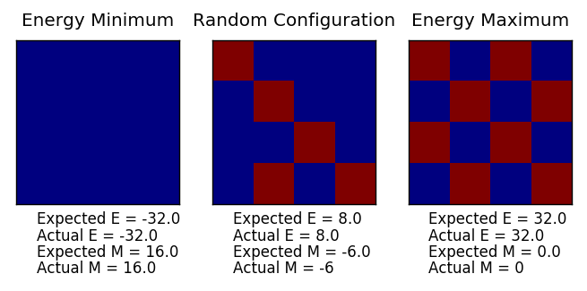
TASK: The code is checked below:

The Monte Carlo Algorithm

To calculate the average energy and magnetization using the ensemble average equations would involve calculating the two parameters for every single possible configuration of the lattice. For a system with 100 spins, there are 2¹⁰⁰ = 1.27 x 10³⁰possible configurations (since the multiplicity W = n^N, where n is two due to there being an up and down spin, and N is the amount of spins in the lattice).

TASK: Assuming it is possible to calculate the magnetization and energy of 1 x 10⁹ configurations per second, it would still take 1.27 x 10²¹ seconds to calculate the entire sum to get the averages $⟨ E ⟩, ⟨ M ⟩$ . That's approximately 10¹³ years, which is contextually a thousand times longer than the current age of the universe and all that has ever transpired, and this computation would be just for one temperature.

JC: Correct.

Since it is virtually impossible to analyse all the configurations of larger lattices, a Monte Carlo algorithm was used to sample configurations which did not have very low Boltzmann factors, thereby sampling configurations that would contribute the most to the average. This importance sampling eliminates a large amount of configurations of the ensemble that would have contributed barely anything to the averages, but together would have severely hampered computational efficiency.

TASK: The code for the Monte Carlo algorithm is implemented above (montecarlostep()) with the energy() and magnetization() functions. The statistics() function was also implemented above.

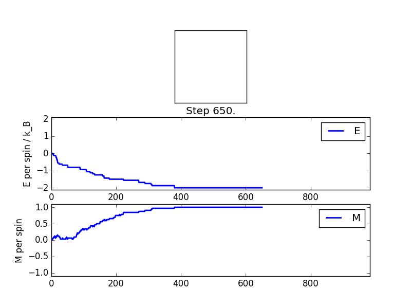
TASK: The temperature is set as T = 1.0, which is below T_C. At this temperature spontaneous magnetization is expected to happen after a certain period of time since the Monte Carlo algorithm favors lower energy states generally (in the algorithm, only one conditional needs to be satisfied in order to accept a lattice with lower energy, and the Boltzmann distribution used by the algorithm favors populating lower energy states). Lower energy states have more spins in parallel and produce magnetism.

This is related to the earlier discussion on the competition between energy and entropy; at lower temperatures than the Curie Temperature there isn't enough energy to flip spins, so lowering the energy by having spins all at parallel is what dominates the behavior of the lattice.

After the magnetization and energy (per spin) of the simulation stabilized after a certain number of Monte Carlo steps, the outputs of the statistics() function were recorded as below.

Number of steps: 670, Averaged quantities: E =  -1.61156716418, E*E =  2.84395988806, M =  0.766884328358, M*M =  0.694190181903

Since the algorithm starts from a randomly generated lattice, it is expected that the system takes a certain number of Monte Carlo steps before it settles into an equilibrium state (shown here as taking about 400 steps). The equilibrium state has all spins in parallel at the lowest energy state as expected.

Accelerating energy and magnetization calculations

A script was used to check the average time taken to complete a computation of 2000 Monte Carlo steps using the previous code (labelled Pre-Accel)

To hasten the computation time, the energy() and magnetization() functions were changed as below.

import numpy as np
from copy import copy,deepcopy

'''
     def energy(self):
         "Return the total energy of the current lattice configuration."
        
         M=self.lattice
         #J is included if it is a parameter that ever needs editing
        J=1.0
         energy=0.0
         #multiply the default lattice by its rolled forms in the four directions
        energy+=(np.sum(np.multiply(M, np.roll(M,1,axis=1)+np.roll(M,-1,axis=1)+np.roll(M,1,axis=0)+np.roll(M,-1,axis=0) )))/(-2)
        return energy
         
     def magnetisation(self):
         "Return the total magnetisation of the current lattice configuration."
        return np.sum(self.lattice)
 '''

JC: Do you need to do roll 4 times in the energy calculation? You can do it just once horizontally and once vertically and then remove the factor of 1/2 from the energy expression as interactions are then not being double counted.

The same computation was then tested using the modified code (labelled Post-Accel), resulting in a significant decrease in the computation time (from almost 10 seconds to just under half a second).

Energy and Magnetization as Functions of Temperature (II)

Discarding transient values

TASK: The Monte Carlo simulation starts from a random lattice configuration and settles into an equilibrium after a certain number of algorithm steps. After observing the behavior of the Monte Carlo simulation on an 8 x 8 lattice using 150000 time steps at differing temperatures, it was seen that equilibrium was reached after about 2000 Monte Carlo steps when T = 1.0. At higher temperatures such as T = 5.0, the values oscillate around a stable mean, and this mean reached equilibrium even faster than 2000 steps. The figures below show the simulations at temperatures 1.0 and 5.0 reaching equilibrium.

Using these simulations as a guide, it was then decided to exclude the values from the first 10000 algorithm steps so as to only capture values at equilibrium. 10000 steps was more than enough to remove any transient values while still being small enough to leave 140000 values for the average. This is expressed in the cut_off variable written in the altered code below:

JC: Did you see how long other lattice sizes or lattices at other temperatures took to equilibrate? You should check that a 32x32 lattice will also have equilibrated in this time.

import numpy as np
from copy import copy,deepcopy

class IsingLattice:
    
    #contains list of running averages
    E = 0.0
    E2 = 0.0
    M = 0.0
    M2 = 0.0
    
    n_cycles = 0
    #specifies amount of initial values to be cut-off, as estimated from test simulations
    cut_off=10000
    
    
    def __init__(self, n_rows, n_cols):
        self.n_rows = n_rows
        self.n_cols = n_cols
        self.lattice = np.random.choice([-1,1], size=(n_rows, n_cols))

    def energy(self):
        "Return the total energy of the current lattice configuration."
        
        M=self.lattice
        #J is included if it is a parameter that ever needs editing
        J=1.0
        energy=0.0
        #multiply the default lattice by its rolled forms in the four directions
        energy+=(np.sum(np.multiply(M, np.roll(M,1,axis=1)+np.roll(M,-1,axis=1)+np.roll(M,1,axis=0)+np.roll(M,-1,axis=0) )))/(-2)
        return energy
        
    def magnetisation(self):
        "Return the total magnetisation of the current lattice configuration."
        return np.sum(self.lattice)

    def montecarlostep(self, T):
        "Run one Monte-Carlo step on the lattice system"
        energy = self.energy()
        #the following two lines will select the coordinates of the random spin for you
        random_i = np.random.choice(range(0, self.n_rows))
        random_j = np.random.choice(range(0, self.n_cols))
        #the following line will choose a random number in the rang e[0,1) for you
        random_number = np.random.random()
        
        #function begins here
        #create a copy of the current lattice, to take advantage of the class attributes
        a1=deepcopy(self)
        #change one of its spins
        a1.lattice[random_i,random_j]=(-1)*(a1.lattice[random_i,random_j])
        
        #get the energy difference as a conditional.
        DE=a1.energy()-energy
        if DE<0:
                self.lattice=a1.lattice
        else:
                if random_number<=(np.exp(-DE/T)):
                        self.lattice=a1.lattice
        #monte carlo main cycle complete
        
        #to then determine whether the energy is added into the running sum, it is checked whether it has past the cut-off threshold
        if self.n_cycles>self.cut_off:
            
            self.E+=self.energy()
            self.E2+=(self.energy())**2
            self.M+=self.magnetisation()
            self.M2+=(self.magnetisation())**2
        
        #cycles are counted regardless of threshold
        self.n_cycles+=1
            
        return self.energy(),self.magnetisation()

    def statistics(self):
        "Returns values of the average energy and magnetisation"
        no=self.n_cycles
        
        #we assign the cutoff to the statistics function
        no2=self.n_cycles-self.cut_off
        
        #print out number of steps
        print("Number of steps: "+str(no))
        
        #prints out cut off value assigned for reference
        print("Cut off: "+str(self.cut_off))
        
        #returns average calculated with cut off value taken into account
        return self.E/no2,self.E2/no2,self.M/no2,self.M2/no2,self.n_cycles

JC: Cut off is well implemented in the code.

Showing the phase transition by plotting the average energy/magnetization against temperature

With the algorithm fully functional, the (importance sampled) ensemble average of the energy and magnetization could be calculated for different temperatures and plotted.

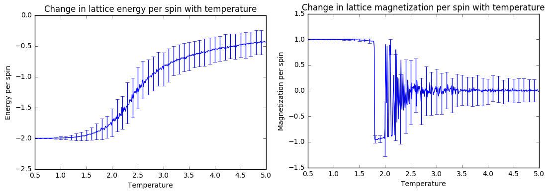
TASK: The average energy and magnetization of an 8 x 8 lattice was calculated for a temperature range of 0.5 to 5.0 using 150000 Monte Carlo steps (with 10000 initial steps excluded from the averaging) and with a step size of 0.01 for the temperature.

The error bars used were calculated from the square root of the variance of E and M. The variance is related to the average through the following equation:

$V a r [X] = ⟨ X^{2} ⟩ - (⟨ X ⟩)^{2}$

As can be seen from the magnetization graph, the magnetization per spin drops from |M| = 1 to approximately zero (the phase transition) between the temperature range of 2.0 < T < 2.5. It can at least be inferred that the Curie Temperature is in that temperature range.

The plots were made using the code below:

import matplotlib.pyplot as plt
import numpy as np

#import all the data
 c=np.loadtxt("8x8_0.01.dat", delimiter=' ')
 
 #assign the data and properties into lists (which will be used more effectively later for multiple lattices)
lat=[c]
siz=[64]
name=['8x8']

#labelling
 plt.xlabel('Temperature')
 plt.ylabel('Energy per spin')
 count=0
 
 #loops once to plot for one type of lattice (8x8)
for i in lat:
    
     #assign all parameters
     T,E,E2,M,M2=i[:,0],i[:,1],i[:,2],i[:,3],i[:,4]
    
     #variances for errors
     varE=E2-(E**2)
     varM=M2-(M**2)
     
     #depending on the y-array chosen, the energy and magnetizations can be plotted
    plt.errorbar(T,E/(siz[count]),yerr=varE**0.5/(siz[count]),errorevery=10,label=name[count])
    count+=1
     
 plt.legend(loc=2)
 plt.title('Energy per spin vs Temperature (8x8)')
 plt.show()

Effects of Lattice Size

TASK: The average magnetization and energies were calculated at differing temperatures for different lattice sizes, and the results are shown below:

JC: Graphs and error bars look good.

The error bars are similarly calculated using the square root of the variances, and the step size for the temperature was 0.01 for each.

Smaller lattice sizes (such as 2 x 2 and 4 x 4) are subject to large amounts of fluctuations and have smaller Curie Temperatures, since there isn't much energy needed to flip so few spins. Their fluctuations are also captured by their calculated error bars which are much higher than those of larger lattice sizes. In fact, the magnetization plots begin to converge with larger lattice sizes, and we will return to this point when comparing the energy plots.

Near the Curie Temperature, which is the temperature for a phase transition, the entropic and energetic forces are almost equal, so the system will fluctuate largely throughout the lattice. A large enough lattice would be needed to simulate these long range fluctuations correctly and reduce the noise around the transition temperature. As can be seen from the above plots, lattice sizes at 2 x 2 and 4 x 4 are poor choices for modelling these fluctuations as they get extremely noisy near T_C and they don't have a large amount of spins, so it's easier for these lattices to oscillate wildly between maximum energy and maximum entropy even in a temperature range near the transition temperature (where neither energy nor entropy should be at a maximum).

To see which of the larger lattice sizes would be adequate to map the long range fluctuations, a plot of the average energy per spin dependence on temperature was made for comparing all lattice sizes below:

Similar to the magnetization, the curves begin to converge at larger lattice sizes. From this plot, it would seem that a 16 x 16 lattice size is adequate to express the energy phase transition and the long range fluctuations, since a lattice size of 32 x 32 doesn't change the curve very much by comparison. Choosing a 32 x 32 lattice would help to reduce the errors though, especially for the magnetization curve (which has more smoother regions when compared to 16 x 16), and would make it easier to identify T_Cwith better precision.

JC: Good analysis.

The code used to make all the above graphs is shown below:

import matplotlib.pyplot as plt
import numpy as np

#import all the data as one
 a=np.loadtxt("2x2_0.01_50ksteps.dat", delimiter=' ')
 b=np.loadtxt("4x4_0.01_50k.dat", delimiter=' ')
 c=np.loadtxt("8x8_0.01.dat", delimiter=' ')
 d=np.loadtxt("16x16_0.01.dat", delimiter=' ')
 e=np.loadtxt("32x32_0.01.dat", delimiter=' ')
 
 #assign the data and properties into lists 
lat=[a,b,c,d,e]
siz=[4,16,64,16**2,32**2]
name=['2x2','4x4','8x8','16x16','32x32']

#labelling can be changed to suit the plot
plt.xlabel('Temperature')
plt.ylabel('Energy per spin')
count=0

#loops to plot multiple lattices
 for i in lat:
     
     #assign all parameters
     T,E,E2,M,M2=i[:,0],i[:,1],i[:,2],i[:,3],i[:,4]
    
     #variances for errors
     varE=E2-(E**2)
     varM=M2-(M**2)
     
     #depending on the y-array chosen, one can choose to plot either magnetization or energy (with error bars)
    plt.errorbar(T,E/(siz[count]),yerr=varE**0.5/(siz[count]),errorevery=10,label=name[count])
    count+=1
     
 plt.legend(loc=2)
 plt.title('Energy per spin vs Temperature (32x32)')
 plt.show()

Heat capacity and the Curie Temperature

TASK: By definition, the heat capacity is:

$C = \frac{\partial ⟨ E ⟩}{\partial T}$

The equation of the average energy was given as:

$⟨ E ⟩ = \frac{\sum_{α} E (α) e^{\frac{- E (α)}{k_{B} T}}}{\sum_{α} e^{\frac{- E (α)}{k_{B} T}}}$

With the general partition function explicitly written out. The partition function represents the sum of all the probabilities of being in different energy states. We use the quotient rule to arrive at the following stage:

$\frac{\partial ⟨ E ⟩}{\partial T} = \frac{(\sum_{α} e^{\frac{- E}{k T}}) (\frac{1}{k T^{2}} \sum_{α} E^{2} e^{\frac{- E}{k T}}) - (\sum_{α} E e^{\frac{- E}{k T}}) (\frac{1}{k T^{2}} \sum_{α} E e^{\frac{- E}{k T}})}{(\sum_{α} e^{\frac{- E}{k T}})^{2}}$

$\frac{\partial ⟨ E ⟩}{\partial T} = \frac{1}{k T^{2}} ⟨ E^{2} ⟩ - \frac{1}{k T^{2}} (⟨ E ⟩)^{2}$

This can be recognized as the form of the variance of the energy (multiplied by 1/kT²)

$\frac{\partial ⟨ E ⟩}{\partial T} = \frac{V a r [E]}{k T^{2}} = C$

JC: Good, clear derivation.

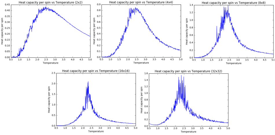
The heat capacity reaches a maximum value at the Curie Temperature, so plots of the heat capacity versus temperature were made to try and find T_C.

Since the Curie Temperature seemed lower for smaller lattices in the previous section, one would try and infer the same behavior from the peaks of the heat capacity plots shifting depending on lattice size. Unfortunately the peaks are too noisy to properly determine the Curie Temperature. Surprisingly the larger lattices (e.g. 32 x 32) have what seem to be the noisiest peaks, which is the opposite trend observed for the magnetization and energy graphs. This is because for an infinite lattice system, the heat capacity actually approaches infinity when approaching T_C (the plot approaches a Delta function), and so as our finite lattices get larger they get closer to an infinite lattice and begin to exhibit more Delta-like peaks near T_C, leading to sharper and what seem to be noisier peaks near T_C as observed. Literature plots have shown that lattice sizes of 256 x 256 would produce really sharp Delta-like peaks.^[1]

JC: The heat capacity diverges (goes to infinity) at Tc for an infinite lattice, but it does not resemble a delta function, which is zero everywhere except for the peak.

A polynomial fit needs to be made for these peaks to get a more precise value of the Curie Temperature, and this is performed in the next section.

The code used to plot the heat capacity graphs is shown below:

import matplotlib.pyplot as plt
import numpy as np

#import all the data as one
 a=np.loadtxt("2x2_0.01_50ksteps.dat", delimiter=' ')
 b=np.loadtxt("4x4_0.01_50k.dat", delimiter=' ')
 c=np.loadtxt("8x8_0.01.dat", delimiter=' ')
 d=np.loadtxt("16x16_0.01.dat", delimiter=' ')
 e=np.loadtxt("32x32_0.01.dat", delimiter=' ')
 
 #assign the data and properties into lists 
lat=[a,b,c,d,e]
siz=[4,16,64,16**2,32**2]
name=['2x2','4x4','8x8','16x16','32x32']

#labelling can be changed to suit the plot
plt.xlabel('Temperature')
plt.ylabel('Heat capacity per spin')
count=0

#loops to plot multiple lattices
 for i in lat:
     
     #assign all parameters
     T,E,E2,M,M2=i[:,0],i[:,1],i[:,2],i[:,3],i[:,4]
    
     #variances for heat capacity
     varE=E2-(E**2)
     varM=M2-(M**2)
     
     #the heat capacity
     C=varE/(T**2)
     
     #plotting heat capacity
     plt.plot(T,C/(siz[count]),label=name[count])
    count+=1
     
 plt.legend(loc=2)
 plt.title('Heat capacity per spin vs Temperature (32x32)')
 plt.show()

Finding the Curie Temperature

Comparing Python data with C++ data

TASK: Data files from a simulation run on C++ were provided and used to similarly plot the energy, magnetization and heat capacity as functions of temperature. The plots were compared to the previous Python plots and it was seen that the peaks for the C++ data were clearer (had less noise) in comparison to their Python counterparts. It could then be more clearly seen that the heat capacity peak was indeed shifting to lower temperatures with increasing lattice sizes. Below are comparison plots of the Python and C++ data for a lattice size of 32 x 32.

For magnetization, energy and heat capacity, the C++ curves look smoother and have less noise. The comparison plots were made using the code below:

import matplotlib.pyplot as plt
import numpy as np

lat_p=np.loadtxt("16x16_0.01.dat", delimiter=' ') #python
lat_c=np.loadtxt("16x16.dat", delimiter=' ') #c

n=16**2 #lattice size, which is changeable

#labelling
 plt.xlabel('Temperature') 
 plt.ylabel('Heat capacity per spin')
 plt.title('Heat capacity per spin comparison (16x16)')
 
 #plots (the y-array can be changed to compare a different parameter)
plt.plot(lat_c[:,0],lat_c[:,5],label='C++ plot')
plt.plot(lat_p[:,0],((lat_p[:,2]-(lat_p[:,1])**2)/((lat_p[:,0])**2))/n,'-',label='Python plot')

plt.legend(loc=1)

plt.show()

Polynomial fits to determine T_C from C

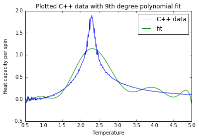
TASK: Using the C++ data, polynomials were fitted to the heat capacity vs temperature plots to find the peak temperature (and hence T_C). The script below was used to perform a 9th degree polynomial fit.

import numpy as np
import matplotlib.pyplot as plt

data = np.loadtxt(...) #assume data is now a 2D array containing two columns, T and C
T = data[:,0] #get the first column
C = data[:,1] # get the second column

#first we fit the polynomial to the data
 fit = np.polyfit(T, C, 9) # fit a ninth order polynomial
  
 #now we generate interpolated values of the fitted polynomial over the range of our function
T_min = np.min(T)
T_max = np.max(T)
T_range = np.linspace(T_min, T_max, 1000) #generate 1000 evenly spaced points between T_min and T_max
fitted_C_values = np.polyval(fit, T_range) # use the fit object to generate the corresponding values of C

#fixing axes and labels
 plt.xlabel('Temperature')
 plt.ylabel('Heat capacity per spin')
 plt.plot(T,C,label='data')
 plt.plot(T_range,fitted_C_values,label='fit')
 plt.legend()
 plt.show()

The result is shown below for fitting a 32 x 32 lattice, and as can be seen the fit still doesn't precisely reflect the data. However, the important point is that the maximum of the fitted polynomial corresponds quite well to the temperature of the C++ data maximum, so with more improvements the polynomial fit can be made to precisely determine T_C.

JC: What about using a higher degree polynomial for the fitting?

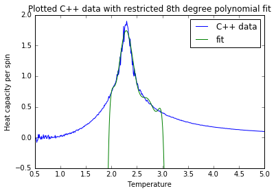
TASK: A more accurate polynomial fit could be attained when the temperature range used for the fit was restricted to near the peak within the C++ data. The code used for this restricted fitting is shown below:

import numpy as np
import matplotlib.pyplot as plt

data = np.loadtxt(...) #assume data is now a 2D array containing two columns, T and C
T = data[:,0] #get the first column
C = data[:,1] # get the second column

#choose a range to fit from
 Tmin = 2
 Tmax = 3
  
 selection = np.logical_and(T > Tmin, T < Tmax) #choose only those rows where both conditions are true
 peak_T_values = T[selection]
 peak_C_values = C[selection]
  
  
 #we fit the polynomial to this range only
fit = np.polyfit(peak_T_values, peak_C_values, 8)

#now we generate interpolated values of the fitted polynomial over the range of our function
T_min = np.min(T)
T_max = np.max(T)
T_range = np.linspace(T_min, T_max, 1000) #generate 1000 evenly spaced points between T_min and T_max
fitted_C_values = np.polyval(fit, T_range) # use the fit object to generate the corresponding values of C

#fixing axes and labels
 plt.xlim(0.5,5.0)
 plt.ylim(-0.5,2)
 plt.xlabel('Temperature')
 plt.ylabel('Heat capacity per spin')
 plt.title('Plotted C++ data with restricted 8th degree polynomial fit')
 plt.plot(T,C,label='C++ data')
 plt.plot(T_range,fitted_C_values,label='fit')
 plt.legend()
 plt.show()

The result is that with almost the same polynomial degree (8th), the fit almost exactly matches the peak of the C++ data as shown below for a 32 x 32 lattice (when the fit was chosen for a temperature range 2.0 < T < 3.0)

Finding T_C for an infinite lattice using the scaling relation

Previously it was seen that T_C begins to converge to a certain value with increasing lattice size, so it can be assumed that for a lattice of infinite size the T_C converges to a certain value. This represents the Curie Temperature for a 2D Ising lattice which we've been trying to determine. The scaling relation^[2] can be used to determine this T_C,∞, which is the Curie Temperature for an infinite 2D lattice:

$T_{C, L} = \frac{A}{L} + T_{C, \infty}$

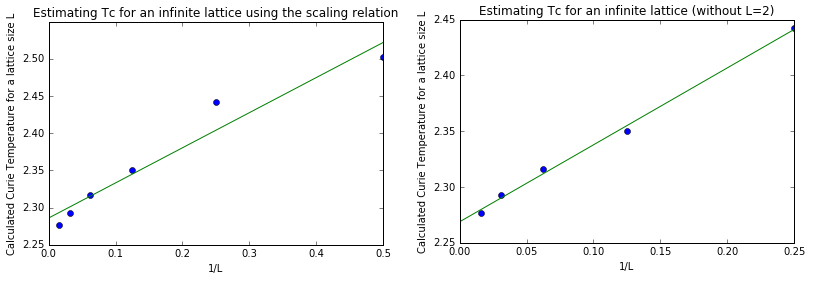
TASK: Therefore a linear fit of T_C,L against 1/L would give the Curie Temperature for an infinite lattice as its intercept. The plots were carried out below:

The code used to make these plots is given below:

import numpy as np
import matplotlib.pyplot as plt

data = np.loadtxt("peaks2.csv", delimiter=',') #assume data is now a 2D array containing two columns, L and T
Lr = 1/data[:,0] #get the first column
T = data[:,1] # get the second column

#we plot a linear fit
 fit = np.polyfit(Lr, T, 1)
 
 #now we generate interpolated values of the fitted line over the range of our function
Lr_min = np.min(Lr)
Lr_max = np.max(Lr)
Lr_range = np.linspace(0, Lr_max, 1000) #set the minimum value to zero and generate an intercept as Tc,inf

fitted_T_values = np.polyval(fit, Lr_range)# use the fit object to generate the corresponding values of T

#fixing axes and labels
 plt.plot(Lr,T,'o')
 plt.plot(Lr_range,fitted_T_values)
 plt.show()
 
 print(np.min(fitted_T_values)) #print intercept value for readout

The initial linear fit (left) gave an intercept of T = 2.286, but this was still including the data of a 2 x 2 lattice. Since that point seems anomalous compared to the other lattice sizes, as well as the fact that a 2 x 2 lattice doesn't accurately represent physical systems since its prone to flipping states regardless of temperature (unless near absolute zero), it was excluded from the fit (which gave the graph on the right). Under the new fit, we have the estimate of T_C,∞ to be:

T_C,∞= 2.2688

JC: Good idea to remove the 2x2 data from the fit.

The analytical solution^[3] in the literature (keeping the reduced units k_B = J = 1.0) eventually shows the value to be:

T_{C,∞, lit} = 2.2692

Conclusion

As can be seen, the numerical result and analytical result have a surprisingly very strong correspondence. This shows that the importance sampling of the Monte Carlo algorithm (run under more steps using the C++ code) is very effective in obtaining quite an accurate representation of the ensemble average (not the time average, which was not taken at all in this work). The success of the algorithm would allow it to be deployed against systems with no analytical solution so that it can compute properties such as the Curie Temperature reliably, and the 3D Ising lattice is still such a system with no analytical solution to its partition function.

Possible major sources of error in the estimate could arise from using lattices that are too small to exhibit realistic behavior within the linear scaling relation. A good example was the exclusion of the 2 x 2 lattice data, which lead to an even more accurate estimate of the Curie Temperature compared to the literature. Perhaps if the 4 x 4 lattice was also excluded, the estimate would become more accurate. Similarly, including more data points from much larger lattices would increase the accuracy of the estimate.

Bibliography

↑ Wang, Fugao & Landau, D. P. (2001). Efficient, Multiple-Range Random Walk Algorithm to Calculate the Density of States. Phys. Rev. Lett., 86, 2050-2053.
↑ V.B. Andreichenko, Vl.S. Dotsenko, W. Selke, J.-S. Wang, Monte Carlo study of the 2D Ising model with impurities, Nuclear Physics B, Volume 344, Issue 3, 1990, Pages 531-556, ISSN 0550-3213, http://dx.doi.org/10.1016/0550-3213(90)90669-5. (http://www.sciencedirect.com/science/article/pii/0550321390906695)
↑ Onsager, Lars (1944). Crystal Statistics. I. A Two-Dimensional Model with an Order-Disorder Transition. Phys. Rev., 65, 117-149.

[1] Wang, Fugao & Landau, D. P. (2001). Efficient, Multiple-Range Random Walk Algorithm to Calculate the Density of States. Phys. Rev. Lett., 86, 2050-2053.

[2] V.B. Andreichenko, Vl.S. Dotsenko, W. Selke, J.-S. Wang, Monte Carlo study of the 2D Ising model with impurities, Nuclear Physics B, Volume 344, Issue 3, 1990, Pages 531-556, ISSN 0550-3213, http://dx.doi.org/10.1016/0550-3213(90)90669-5. (http://www.sciencedirect.com/science/article/pii/0550321390906695)

[3] Onsager, Lars (1944). Crystal Statistics. I. A Two-Dimensional Model with an Order-Disorder Transition. Phys. Rev., 65, 117-149.

[1]

[2]

[3]