Talk:Mod:tsf1234
NJ: A good effort, well done. Take care with your written communication, there are a few sections of text which are difficult to follow. Specific comments below.
Third Year Chemistry Lab
CID=00881295
Introduction to Molecular Dynamics Simulation

For the file HO.xls, three columns " Analytical" , "Error" and " Energy" are completed.
Analytical value can be found by using the equation x(t)= A cos( wt + Φ) , since w= 1, A= 1 and Φ is equal to 0 hence the x= cos( t) , where t= time.
Error can be found by using absolute function in excel to eliminate the +/- sign. The error value is the difference between analytical value and given value of x(t).
A graph of position of maxima in the error column as a function of time is plotted(Figure 1.1)

Energy of the system including both potential energy and kinetic energy.
E = 1/2 mv2 (kinetic energy)+ 1/2 kx2 (potential energy) , where v(t) is the value given.
As time increases, the maximum error increases.
According to the conservation of energy , energy should be constant in the system. However, the graph of energy versus time(shows that there is a very small fluctuation in energy. The energy varies periodically with time(Figure 1.2).
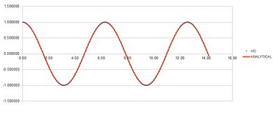
Any time step equal 0.2 or below can be ensure that the total energy does not varies by more than 1% over the course of simulation by calculating the 0.1% of total energy. The smaller the time step, the more accurate is the result , the energy is more constant over the system. Total energy of a system is important to be monitored because it can shows how closely is the system to the reality. If the total energy does not varies a lot over the course of simulation, it is closely obeying the law of conservation of energy.
Introduction to molecular dynamics simulation
Lennard-Jones interaction measures the interaction between a pairs of atoms and it includes both repulsive and attractive term.

TASK: For a single Lennard-Jones interaction, , find the separation, r_0, at which the potential energy is zero. What is the force at this separation? Find the equilibrium separation, r_{eq}, and work out the well depth (\phi\left(r_{eq}\right)). Evaluate the integrals.
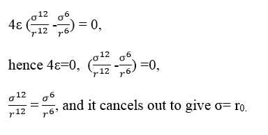
When the potential energy is zero,
Force of separation can be calculated by differentiate the Lennard-Jones interaction with respect to r.
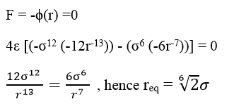
At equilibrium separation, force = 0
NJ: r is a variable, sigma is a constant. You need to replace r by sigma, not the other way around.
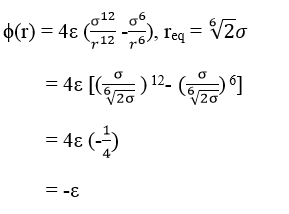
Well depth, Φ(req) can be found by substitute the equilibrium separation into the Lennard-Jones interaction equation.
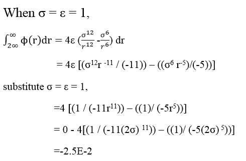
Evaluate the integrals.
When σ = ε = 1,
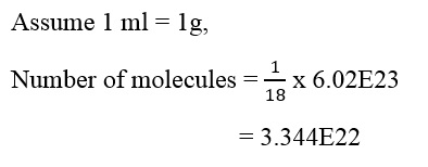
Estimate the number of water molecules in 1ml of water under standard conditions. Estimate the volume of water molecules under standard conditions
Estimate the volume of water molecules under standard conditions
TASK: Consider an atom at position (0,0,0) in a cubic simulation box which runs from (0,0,0) to (1,1,1). In a single time step, it moves along the vector (0.7, 0.6, 0.2). At what point does it end up, after the periodic boundary conditions have been applied?.
The atom will end up at position (0.2,0.1,0.7). For periodic boundary conditions, we assume same number of atoms will confine in a box, which means a box will extend to its surrounding infinitely( to all direction). When one atom in a reference box moves to the right of the box, the periodic boundary condition indicates that another atom from box on the left will now enter the reference box. In this case, the number of atoms in all boxes will be fixed. Starting from the position(0.5,0.5,0.5), the atom moves via the x-axis by 0.7, y-axis by 0.6 and z axis by 0.2.
Position of atom can be calculated via:
(A box has a dimension of 1 X 1 X 1, when the value of vector exceeds 1.0, it indicate the atom has moved to another box.)
0.5+0.7-1.0=0.2
0.5+0.6-1.0=0.1
0.5+0.2=0.7
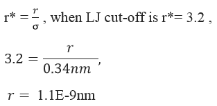
TASK: The Lennard-Jones parameters for argon are \sigma = 0.34\mathrm{nm}, \epsilon\ /\ k_B= 120 \mathrm{K}. If the LJ cutoff is r^* = 3.2, what is it in real units? What is the well depth in \mathrm{kJ\ mol}^{-1}? What is the reduced temperature T^* = 1.5 in real units?
Given the Lennard-Jones parameters for argon are σ = 0.34nm, ε/K_B =120K,
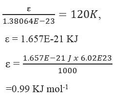
Given that Boltzmann constant is 1.38064E-23m2 kg s-2 k-1, well depth can be calculated by using ε/K_B =120K
To get ε in KJ mol-1, the value is multiplied by Avogadro number and divide by 1000.
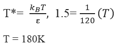
When reduced temperature T = 1.5 in real units,
Equilibrium
TASK: Why do you think giving atoms random starting coordinates causes problems in simulations? Hint: what happens if two atoms happen to be generated close together?
Problems might occurred if random starting coordinates are set during the simulation. If two atoms happen to be generated too close together, it might undergo repulsion and the atoms arrangement will be too alike as solid. If it is too far away from each other, it might assemble the atoms arrangement of gas instead of liquid.
NJ: No, the random configuration is much more liquid like than a crystal. If two atoms are very close together, there will be very large forces between them.
TASK: Satisfy yourself that this lattice spacing corresponds to a number density of lattice points of . Consider instead a face-centred cubic lattice with a lattice point number density of 1.2. What is the side length of the cubic unit cell?
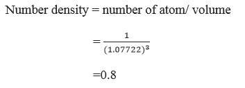
Number density corresponds to number of lattice points per unit volume.
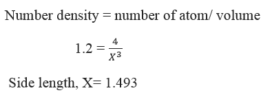
For a face centered cubic, there are 4 lattice points(1/8*1 + 1/2*6 = 4 )and hence 4 atoms in a unit cell.
When the face-centered cubic lattice has a lattice point density of 1.2,
TASK: Consider again the face-centred cubic lattice from the previous task. How many atoms would be created by the create_atoms command if you had defined that lattice instead?
create_atoms 1 box
Our box contains 1000 (10x10x10) unit cells of this lattice, and so contains 1000 lattice points.
1 box contains 1000 unit cells and 1000 lattice points, and due to the fact that 4 atoms are placed in a box, 4000 atoms will be created.
TASK: Using the LAMMPS manual, find the purpose of the following commands in the input script:
mass 1 1.0
pair_style lj/cut 3.0
pair_coeff * * 1.0 1.0
Mask 1 1.0
This command is used to set the mass of the atom in the lattice box by specify the type and mass of atom. Value 1 between mass and 1.0 corresponds to the type of atom used. Value 1.0 corresponds to value of mass of atom
pair_style lj/cut 3.0
This indicates that only Lennard Jones interaction between pair of atoms in distance of 3 units will be considered. Any distance more than 3 units will be cut off which means the potential energy due to interaction will be zero.
pair_coeff * * 1.0 1.0
** in the middle corresponds to the types of atoms can be anything from 1 to N. 1.0 1.0 is the value for coefficient which in this case corresponds to sigma and Φ(well depth) that based in Lennard-Jones potential. Sigma corresponds to the distance when the potential energy between particle is zero.
TASK: Given that we are specifying Xi(0) and Vi(0), which integration algorithm are we going to use?
Velocity verlet algorithm should be used.
The second line (starting "variable timestep...") tells LAMMPS that if it encounters the text ${timestep} on a subsequent line, it should replace it by the value given. In this case, the value ${timestep} is always replaced by 0.001. In light of this, what do you think the purpose of these lines is? Why not just write:
timestep 0.001
run 100000
This is to make sure the simulation time will be constant for comparison of different time step for a energy versus time plot. If the time is different, the scale for x-axis would be different for different time step. The command is designed such that the number of time step will always change according to the value of time step so that the total simulation time will be 100. The larger the value of time step, the lower the number of time step.
TASK: make plots of the energy, temperature, and pressure, against time for the 0.001 timestep experiment (attach a picture to your report). Does the simulation reach equilibrium? How long does this take? When you have done this, make a single plot which shows the energy versus time for all of the timesteps (again, attach a picture to your report). Choosing a timestep is a balancing act: the shorter the timestep, the more accurately the results of your simulation will reflect the physical reality; short timesteps, however, mean that the same number of simulation steps cover a shorter amount of actual time, and this is very unhelpful if the process you want to study requires observation over a long time. Of the five timesteps that you used, which is the largest to give acceptable results? Which one of the five is a particularly bad choice? Why?
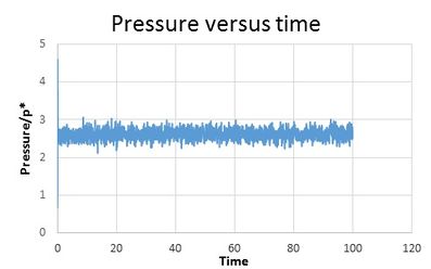
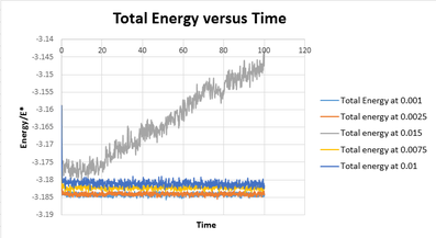
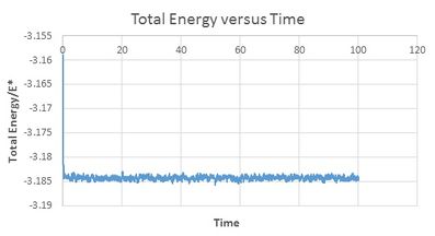
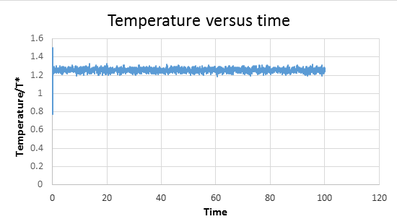
The simulation reach equilibrium because the energy becomes almost constant. It takes a very short period of time for system to go to equilibrium(when the graph starts to show a straight line) , approximately 0.035(in unit of t). According to the figure 1.8, both time step at 0.001 and 0.0025 gives similar result, which both shows smallest fluctuation which obey the law of conservation of energy, and hence gives a minimum error. It is true that smallest time step provides most accurate results. However, given both time step provides similar results, 0.0025 is a better choice because the system that run the time step at 0.0025 will has a longer total simulation time. Time step of 0.015 gives the worst result because energy is not constant throughout the simulation time. Energy increases as time goes by and this deviates from reality.
Running Simulations under specific conditions
TASK: Choose 5 temperatures (above the critical temperature T^* = 1.5), and two pressures (you can get a good idea of what a reasonable pressure is in Lennard-Jones units by looking at the average pressure of your simulations from the last section). This gives ten phase points — five temperatures at each pressure. Create 10 copies of npt.in, and modify each to run a simulation at one of your chosen \left(p, T\right) points. You should be able to use the results of the previous section to choose a timestep. Submit these ten jobs to the HPC portal. While you wait for them to finish, you should read the next section.
Temperatures are set at 1.6, 1.8,2.0,2.2 and 2.4 and pressure are set at 2.5 and 2.7. These 5 different temperatures are run at 2.5p* and 2.7p* respectively and this gives 10 different points.Time step of 0.0025 is set because this gives least fluctuation in the graph of total energy versus time and reasonable longer simulation time according to previous section.
ASK: We need to choose \gamma so that the temperature is correct T = \mathfrak{T} if we multiply every velocity \gamma. We can write two equations:
TASK: Use the manual page to find out the importance of the three numbers 100 1000 100000. How often will values of the temperature, etc., be sampled for the average? How many measurements contribute to the average? Looking to the following line, how much time will you simulate?
The first 100 commands the system to record a time step of 100 . 1000 in the middle corresponds to the number of steps used to to take final average during 100000 time step and 100000 corresponds that system will takes an final average on 100000 time steps. For example, for 5 5 100, the system has a time step of 5, and it will average the value of 95+90+85+80+75 during the 100 time step.
TASK: Use software of your choice to plot the density as a function of temperature for both of the pressures that you simulated. Your graph(s) should include error bars in both the x and y directions. You should also include a line corresponding to the density predicted by the ideal gas law at that pressure. Is your simulated density lower or higher? Justify this. Does the discrepancy increase or decrease with pressure?
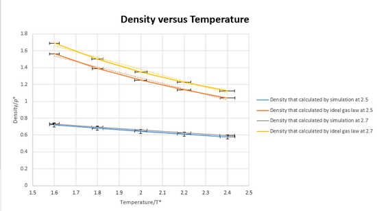
Density can be calculated by,
A plot of p/T(equal to density) versus temperature is plotted on the same graph as the density simulated as a function of temperature.
As seem in figure 1.9, as temperature increases, density decreases. As temperature increases, atoms gain kinetic energy and moves further away from each other and hence density decreases. Pressure is set as constant in this case.
The simulated density is lower that the density that calculated by ideal gas law. According to ideal gas law, there is no forces/ potential energy between the moving atoms. When the atoms get close together, there is no repulsion force. hence the atoms can get closer to each other and the density is higher. Whereas for the case of density that calculated by simulation, the atoms repulse each other and hence the density is lower.
A plot of graph of density versus temperature from the simulated density versus temperature shows a lower discrepancy because when the atoms are closer together at higher pressure, there is repulsion between the atoms,atoms cannot get close together and hence the overall density is very similar for two different pressure.
Error plot at x-axis and y-axis have been plot by using the standard error value that calculated from simulation. There is no error bar shown in the y-axis for density that calculated from ideal gas law.
Calculating heat capacities using statistical physics
TASK: As in the last section, you need to run simulations at ten phase points. In this section, we will be in density-temperature \left(\rho^*, T^*\right) phase space, rather than pressure-temperature phase space. The two densities required at 0.2 and 0.8, and the temperature range is 2.0, 2.2, 2.4, 2.6, 2.8. Plot C_V/V as a function of temperature, where V is the volume of the simulation cell, for both of your densities (on the same graph). Is the trend the one you would expect? Attach an example of one of your input scripts to your report.
Attachment of the script when temperature= 2.2 and density equal to 0.8.
Explaination and detail of the script
<lattice sc 0.8>
Density is set to 0.8. Sc corresponds to solid cubic lattice.
<variable T equal 2.4>
Temperature is changed to 2.4 (which is in reduced unit).
<fix nvt all nvt temp ${T} ${T} ${tdamp}>
Npt has been replaced by nvt because density and temperature are kept constant. Density is indirectly corresponds to volume because number of atoms in the system is fixed.
<unfix nvt fix nve all nve>
This command is used to turn off the command. These command have to be put in lines after the system have been run.)
### MEASURE SYSTEM STATE ###
thermo_style custom step etotal temp press density atoms vol
variable temp equal temp
variable temp2 equal temp*temp
variable N equal atoms
variable N2 equal atoms*atoms
variable etotal equal etotal
variable etotal2 equal etotal*etotal
variable volume equal vol
MEASURE SYSTEM STATE is used to define all the variable that need to be calculated by the system.
fix aves all ave/time 100 1000 100000 v_dens v_temp v_press v_dens2 v_temp2 v_press2 v_etotal v_etotal2
This command is used to calculate the average value of the variable stated.
variable avedens equal f_aves[1]
variable avetemp equal f_aves[2]
variable aveetotal equal f_aves[7]
variable aveetotal2 equal f_aves[8]
For f_aves[X], X corresponds to variable to the right of 100 1000 100000 For example, f_aves[1] corresponds to the first variable to the right of 100 1000 100000 which corresponds to v_dens.
variable heatcapacity equal ${N2}*(${aveetotal2}-${aveetotal}*${aveetotal})/(${avetemp}*${avetemp})
Every variable has to be put in ${} for the system to detect it.
Value of heat capacity cannot be simulated directly but LAMMPS can help to calculated the heat capacity by using this equation,
Since kB is known as 1( in reduced unit), T2, N2, <E2> and <E>^2 have to be calculated by the system to obtain the value of heat capacity.
T2 can be obtained by temp*temp
N2 can be obtained by number of atom*number of atom.
<E2> is the average of total energy*total energy and this represented by aveetotal2 in the script.
<E>^2 is the square of average value of total energy and this can be represented by aveetotal*aveetotal.
print "Averages"
print "--------"
print "Density: ${avedens}"
print "Temperature: ${avetemp}"
print "total energy: ${aveetotal}"
print "total energy: ${aveetotal2}"
print "heatcapacity: ${heatcapacity}"
print "number of atoms: ${N2}"
print "volume: ${volume}"
These section is used to print the variable that have been defined in MEASURE SYSTEM STATE.
### DEFINE SIMULATION BOX GEOMETRY ###
lattice sc 0.8
region box block 0 15 0 15 0 15
create_box 1 box
create_atoms 1 box

### DEFINE PHYSICAL PROPERTIES OF ATOMS ###
mass 1 1.0
pair_style lj/cut/opt 3.0
pair_coeff 1 1 1.0 1.0
neighbor 2.0 bin

### SPECIFY THE REQUIRED THERMODYNAMIC STATE ###
variable T equal 2.4
variable timestep equal 0.0025

### ASSIGN ATOMIC VELOCITIES ###
velocity all create ${T} 12345 dist gaussian rot yes mom yes

### SPECIFY ENSEMBLE ###
timestep ${timestep}
fix nve all nve

### THERMODYNAMIC OUTPUT CONTROL ###
thermo_style custom time etotal temp press
thermo 10

### RECORD TRAJECTORY ###
dump traj all custom 1000 output-1 id x y z

### SPECIFY TIMESTEP ###

### RUN SIMULATION TO MELT CRYSTAL ###
run 10000
unfix nve
reset_timestep 0

### BRING SYSTEM TO REQUIRED STATE ###
variable tdamp equal ${timestep}*100
variable pdamp equal ${timestep}*1000
fix nvt all nvt temp ${T} ${T} ${tdamp}
run 10000
reset_timestep 0
unfix nvt
fix nve all nve

### MEASURE SYSTEM STATE ###
thermo_style custom step etotal temp press density atoms vol
variable dens equal density
variable dens2 equal density*density
variable temp equal temp
variable temp2 equal temp*temp
variable press equal press
variable press2 equal press*press
variable N equal atoms
variable N2 equal atoms*atoms
variable etotal equal etotal
variable etotal2 equal etotal*etotal
variable volume equal vol
fix aves all ave/time 100 1000 100000 v_dens v_temp v_press v_dens2 v_temp2 v_press2 v_etotal v_etotal2
run 100000

variable avedens equal f_aves[1]
variable avetemp equal f_aves[2]
variable avepress equal f_aves[3]
variable aveetotal equal f_aves[7]
variable aveetotal2 equal f_aves[8]

variable heatcapacity equal ${N2}*(${aveetotal2}-${aveetotal}*${aveetotal})/(${avetemp}*${avetemp})

print "Averages"
print "--------"
print "Density: ${avedens}"
print "Temperature: ${avetemp}"
print "pressure: ${avepress}"
print "total energy: ${aveetotal}"
print "total energy: ${aveetotal2}"
print "heatcapacity: ${heatcapacity}"
print "number of atoms: ${N2}"
print "volume: ${volume}"
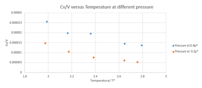
Heat capacity is defined as amount of energy needed to increase the temperature by 1 K (unit: J K-1).
When temperature increases, the internal energy increases as there are more degree of freedom and hence it is harder to increase the heat capacity. It is due to the fact that atoms are far apart from each other and hence it harder for an atom to transfer the energy to neighbor atoms. Hence it is not the trend that to be expected. However, according to the figure 1.10 which shows a plot of Cv/V as a function of temperature shows a different relationship as expected. The graph shows that as temperature increases heat capacity decreases. This might due to the error associated to the simulation.
For solid and liquid, pressure is not an important factor to consider because solid and liquid do not expand much when heat energy increases. However, in the case of heating up gas, work needed to be done to against the pressure and hence generally a higher heat capacity will be observed at a higher temperature.
Structural properties and the radial distribution function
TASK: perform simulations of the Lennard-Jones system in the three phases. When each is complete, download the trajectory and calculate g(r) and \int g(r)\mathrm{d}r. Plot the RDFs for the three systems on the same axes, and attach a copy to your report. Discuss qualitatively the differences between the three RDFs, and what this tells you about the structure of the system in each phase. In the solid case, illustrate which lattice sites the first three peaks correspond to. What is the lattice spacing? What is the coordination number for each of the first three peaks?
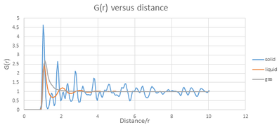
Radial Distribution Relationship describes the relationship between density and distance from a reference particle.
The value for density and temperature can be found from article given in the script[1].
[1] Jean-Pierre Hansen, Loup Verlet , Verlet, Loup, Phys. Rev, 1986, vol 184, 151-161
The graph of g(R)versus distance for solid shows a lot of peaks that which means at a given distance that shows peaks, atoms can be found.For solid, the atoms are closer to each other and it has short range order that atoms are bonded closely.
NJ: The solid also has long range order
Whereas for liquid, there are few peaks only when the distance is less than 4r. The graph approaches to 1 at as longer distance because there is no short range order. NJ: The liquid has short-range, but no long range order
For gas, only 1 peak can be found within the distance and the graph approaches to 1 at a even shorter distance compares with liquid. This indicates that atoms can be only found when r is approximately 1. Atoms can be found around that distance which is due to the attraction between the reference atom to the neighbors atoms.
However, all peaks decreases to g(r)=1 as distance from a reference particle increases.
In the case of solid, the first peaks correspond to the first nearest atoms, second peaks corresponds to the second nearest atoms and third peaks corresponds to third nearest atoms.
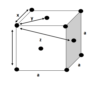
Since this is a face centered cubic structure, the position of the atoms can be found.
Face centered cubic a unit length of a.
Distance of first nearest atoms(x)= , second nearest atoms(y)= a , third nearest atoms(z)=
The distance from atoms to the reference atom can be found from figure 1.11 which is 1.025,1.525 and 1.825(directly read off from the first 3 peaks on the graph.
Distance to the first nearest atoms, r =1.03, =1.0 , a=1.45 ,
Distance to the second nearest atoms, r= 1.53, a = 1.53
Distance to the third nearest atoms, r =1.83,
= 1.83 ,a =1.49
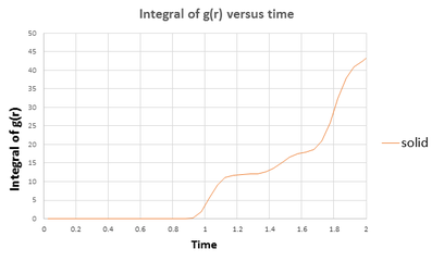
To get a more accurate value, these 3 values are added to get the average value.
(1.45+1.53+1.49/3)
Average lattice spacing , a = 1.5,
NJ: Excellent
The coordination number can be directly read off from the graph of integral of g(r) versus time. The value of integral g(r)(y-axis) at distance r for the first three peaks corresponds to coordination number.
These value are just estimate value.
Coordination number of first peak = 12
Coordination number of second peak= 18
Coordination number of third peak = 32
NJ: You need the difference between each site and the previous one. e.g. first coordination shell: 12; second coordination shell: 18-12 = 6; third coordination shell: 42-18 = 24
Dynamic properties and diffusion coefficients
The diffusion coefficient D can be calculated by using the equation below.

A plot of mean square displacement versus time has been plotted.
Gradient of the graph can be used to find the mean square displacement.
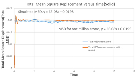

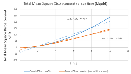
D = 1/6* gradient
| phase | gradient(simulated phase) | D (simulated phase) | gradient(given data) | D(given data) |
|---|---|---|---|---|
| Solid | 6E-08 | 9.6E-08 | 2E-08 | 3.3E-09 |
| Liquid | 1E-02 | 1.7E-03 | 1E-02 | 1.7E-03 |
| Gas | 24.2 | 4.03 | 15.3 | 2.55 |
Table 1 show the gradient from the graph of D versus number of time step of simulated phase and given data for one million atoms.
Diffusion coefficient has a unit of m^2 S-1 according to the equation and hence MSD is plot against time instead of time step.
Mean square displacement for solid is very small because atoms in solid do not move around vigorously, it only vibrates at its own positions. As expected, the distance is small.
TASK: In the theoretical section at the beginning, the equation for the evolution of the position of a 1D harmonic oscillator as a function of time was given. Using this, evaluate the normalised velocity autocorrelation function for a 1D harmonic oscillator (it is analytic!):
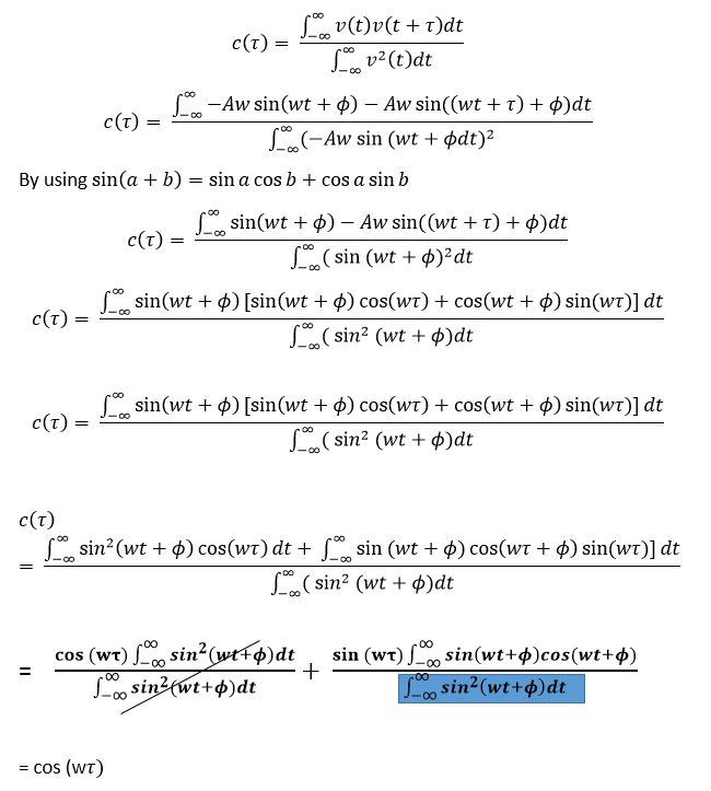
=*The mathematics calculation that highlighted in blue is canceled out because denominator part will add up to a infinite number and hence when the numerator divide by denominator, the whole term cancel out. NJ: in fact, it cancels out because the numerator is zero (it's an odd function).

Task.Velocity autocorrrelation(VACF) can be calcultaed for a 1D harmonic oscillator and the value of c(τ) can be used to plot versus timestep, τ to compare with VACF from the simulation of solid and liquid.
What do the minima in the VACFs for the liquid and solid system represent? Discuss the origin of the differences between the liquid and solid VACFs. The harmonic oscillator VACF is very different to the Lennard Jones solid and liquid. Why is this?
C(τ) = cos(wτ)whereas τ is equal to 0.5π.
For a simple harmonic motion, minimum and maximum corresponding the points when the atoms start to change its position.
As seem in the figure 1.16, the graph for solid oscillates more before the c(τ) comes to zero. C(τ) is a measure of how the velocity at time(τ) related to its previous velocity. Hence when the y-axis of the graph ceases to zero, it indicates that atom at time step(τ) is not related to previous velocity of itself anymore.
Molecules in solid are very close to each others and hence it do not moves freely but merely vibrate forward and backward. In this case, when an atom knock on the other atoms, it change the other atom's velocity and bound back, it is just merely a vibration and hence the velocity will not change much and the velocity will be still related in a short time. Whereas for the case of liquid, it moves more freely as the atoms are not arrange in a close pack manner and atoms in a liquid collide each other more frequently and hence any atoms in liquid has a higher probability to 'lose its memory' and gain a velocity as it change its direction or speed.
Harmonic oscillator VACF varies from Lennard Jones liquid and solid VACF because for harmonic oscillator, atom moves backward and forward without knock on to any other atoms.We treat the whole system as a single atom system.Hence the velocity correlation function just moves like a normal cosine curve, from positive to negative as it changes the direction but it has the same magnitude(velocity is a vector function) which means the velocity of the atom always depend on its previous velocity. Whereas for Lennard Jones liquid and solid, there is interaction between atoms and hence VACF ceases to zero as distance increases.
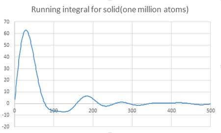
TASK: Use the trapezium rule to approximate the integral under the velocity autocorrelation function for the solid, liquid, and gas, and use these values to estimate D in each case. You should make a plot of the running integral in each case. Are they as you expect? Repeat this procedure for the VACF data that you were given from the one million atom simulations. What do you think is the largest source of error in your estimates of D from the VACF?
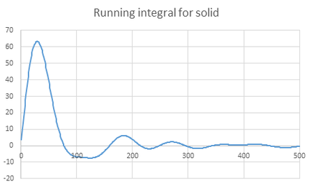
Trapezium is used to estimate the area under curve.
It can be calculated by using the formula below
=0.5*(first value+last value of the y axis)+2*(SUM of 2nd value to 499th value of y axis)*(1(which is the number of time step))
Area under the graph,for solid =-2.495 , liquid= 236.4 and gas = 2867
D = 1/3 * Integral Value
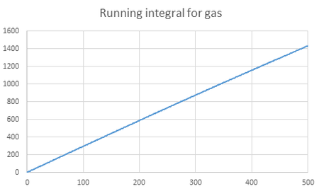
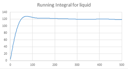
| Phase | Integral value | Value of D |
|---|---|---|
| solid | -2.495 | -0.832 |
| liquid | 236.4 | 78.8 |
| gas | 2867 | 955 |
Table 2 shows the value of integral value and D for simulated phase of solid,liquid and gas.
Value of D for simulated phase of solid, liquid and gas are of expected. Gas should has the highest diffusion coefficient because atoms moves(diffuses) quickly as it poses high kinetic energy in gas phase. From solid to gas, which corresponds to increase in kinetic energy, diffusion coefficient also increases.
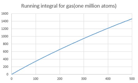
| Phase | Integral value | Value of D |
|---|---|---|
| solid | -2.654 | -0.885 |
| liquid | 245.7 | 81.9 |
| gas | 2930 | 978 |
Table 3 shows the integral value and D for one million atoms.
Value of D for simulated gas, solid and liquid for one million atoms has the very similar result for diffusion coefficient as previous simulation.
VACF value obtained from given data of one million atoms should provide a more accurate result because it obtained higher number of atoms( 1,000,000 versus 3375).
Higher number of atoms will be more representative. Hence, the biggest error for the simulation should be low number of atoms which less representative.
NJ: But is it realistic that it's so much higher? Unfortunately not. Your VACF D is per-timestep, whereas the MSD D is per-time. They differ by a factor of approximately
