Talk:Mod:tonyyang

Comments in red

Introduction

In this experiment, computational molecular dynamic methods involving Velocity-Verlet algorithm and Lennard-Jones potentials were used to model a mono-atomic system. Some of the thermodynamics data was calculated from simulations by using statistical thermodynamics.

Theory

A plot of ERROR against time. The maxima are picked and fitted to a straight line.

In the plot of error against time, the error appears to be oscillating periodically with time. This is because the Velocity-Verlot algorithm assumed constant velocity within each timestep. This is generally a good enough assumption, however, the error will increase when the simple harmonic oscillator is at its maximum acceleration. Therefore, the maxima in error appear periodically (the period is $\pi$). Tick

---

A plot of energy against time at timestep=0.28.

A plot of energy against time at timestep=0.28. The maximum deviation from the average energy does not exceed 1%.

The algorithm used to is not a perfect description for the energy of the system. So if the energy deviates too much from reality then this algorithm is not good enough for the simulation. Although small timestep can produce a better result, the simulation will also take longer. So a good balance between accuracy and time is needed. Tick, could also mention how errors accumulate

---

For $r_0=\sigma$, potential energy $\varphi \left(r_0\right)=4ϵ(\frac{{\sigma }^{12}}{{r_0}^{12}}-\frac{{\sigma }^6}{{r_0}^6})=4ϵ(1-1)=0$.

And the force:

$\begin{array}{rl}F\left(r\right)& =-\frac{\mathrm{d}U\left(r\right)}{\mathrm{d}r}\\ & =-\frac{\mathrm{d}\left(4ϵ(\frac{{\sigma }^{12}}{r^{12}}-\frac{{\sigma }^6}{r^6})\right)}{\mathrm{d}r}\\ & =-4ϵ(-12\frac{{\sigma }^{12}}{r^{13}}-(-6)\frac{{\sigma }^6}{r^7})\\ & =-24ϵ(-2\frac{{\sigma }^{12}}{r^{13}}+\frac{{\sigma }^6}{r^7})(1)\end{array}$

When $r=\sigma$, $F(r)=-24ϵ(-2\frac{1}{r}+\frac{1}{r})=24\frac{ϵ}{r}$. Good

---

At equilibrium separation, $r_{eq}$, force is zero,

$\begin{array}{rl}F(r_{eq})& =-24ϵ(-2\frac{{\sigma }^{12}}{r_{eq}^{13}}+\frac{{\sigma }^6}{r_{eq}^7})=0\\ \frac{{\sigma }^6}{r_{eq}^7}& =2\frac{{\sigma }^{12}}{r_{eq}^{13}}\\ r_{eq}^6& =2{\sigma }^6\\ r_{eq}& =2^{\frac{1}{6}}\sigma \end{array}$

At this separation, the well depth,

$\varphi (r_{eq})=4ϵ(\frac{{\sigma }^{12}}{4{\sigma }^{12}}-\frac{{\sigma }^6}{2{\sigma }^6})=4ϵ(\frac{1}{4}-\frac{1}{2})=-ϵ$

---

$\int \varphi \left(r\right)\mathrm{d}r=\int 4ϵ(\frac{{\sigma }^{12}}{r^{12}}-\frac{{\sigma }^6}{r^6})\mathrm{d}r=4ϵ(-\frac{1}{11}\frac{{\sigma }^{12}}{r^{11}}+\frac{1}{5}\frac{{\sigma }^6}{r^5})$

When $\sigma =ϵ=1.0$, the integral becomes,

$\int \varphi \left(r\right)\mathrm{d}r=-\frac{4}{11r^{11}}+\frac{4}{5r^5}$,

therefore,

$\underset{2\sigma }{\overset{\mathrm{\infty }}{\int }}\varphi \left(r\right)\mathrm{d}r=(-\frac{4}{11{\mathrm{\infty }}^{11}}+\frac{4}{5{\mathrm{\infty }}^5})-(-\frac{4}{11\times 2^{11}}+\frac{4}{5\times 2^5})=-0.0248$

and similarly,

$\underset{2.5\sigma }{\overset{\mathrm{\infty }}{\int }}\varphi \left(r\right)\mathrm{d}r=-0.00818$

$\underset{3.0\sigma }{\overset{\mathrm{\infty }}{\int }}\varphi \left(r\right)\mathrm{d}r=-0.00329$.

As can be seen here, the integral of energy after $3.0\sigma$ is sufficiently small. So it is safe to make $3.0\sigma$ the cut-off point. Correct

---

Number of water molecules in 1mL of water = $\frac{mass}{molarmass}\times N_A=\frac{1\mathrm{g}}{18\mathrm{g}/\mathrm{m}\mathrm{o}\mathrm{l}}\times 6.022\times 10^{23}{\mathrm{m}\mathrm{o}\mathrm{l}}^{-1}=3.35\times 10^{22}$

Volume of 10000 water molecules $=\frac{10000}{N_A}\times \frac{\mathrm{m}\mathrm{o}\mathrm{l}\mathrm{a}\mathrm{r}\mathrm{m}\mathrm{a}\mathrm{s}\mathrm{s}}{\mathrm{d}\mathrm{e}\mathrm{n}\mathrm{s}\mathrm{i}\mathrm{t}\mathrm{y}}=\frac{1000}{6.022\times 10^{23}}\times \frac{18\mathrm{g}/\mathrm{m}\mathrm{o}\mathrm{l}}{1\mathrm{g}/\mathrm{c}{\mathrm{m}}^{\mathrm{3}}}=2.99\times 10^{-19}\mathrm{c}{\mathrm{m}}^{\mathrm{3}}$ Tick

---

(0.5, 0.5, 0.5) + (0.7, 0.6, 0.2) = (1.2, 1.1, 0.7)

But because of the periodic conditions, the atom re-enters the cube one it leaves the cube. So, once its coordinate exceed 1, that coordinate will be reset to 0, ie. co-ordinates modulo 1.

So, the atom ends on (0.2, 0.1, 0.7).

---

$r$ in real unit:

$r=r^{*}\times \sigma =3.2\times 0.34\times 10^{-9}\mathrm{m}=1.09\times 10^{-9}\mathrm{m}$

Well depth in real unit:

$-ϵ=-120\mathrm{K}\times 1.38\times 10^{-23}\mathrm{J}/\mathrm{K}\times 6.022\times 10^{23}=997\mathrm{J}/\mathrm{m}\mathrm{o}\mathrm{l}=0.997\mathrm{k}\mathrm{J}/\mathrm{m}\mathrm{o}\mathrm{l}$

$T$ in real unit: $T=\frac{T^{*}ϵ}{k_B}=1.5\times 120\mathrm{K}=150\mathrm{K}$

Equilibration

When two atoms are close together, they repel each other very strongly and the inter-atomic energy will rise rapidly. By randomly assign coordinates to atoms, the system's internal energy could get unrealistically high and impossible to maintain the required conditions for a certain ensemble.

---

Simple cubic lattice, 1 lattice point per unit cell.

$\mathrm{N}\mathrm{u}\mathrm{m}\mathrm{b}\mathrm{e}\mathrm{r}\mathrm{d}\mathrm{e}\mathrm{n}\mathrm{s}\mathrm{i}\mathrm{t}\mathrm{y}\mathrm{=}\frac{latticepointperunitcell}{volumeofunitcell}=\frac{1}{1.07722^3}=0.800$

Face-centred cubic lattice has 4 lattice points per unit cell.

$\mathrm{U}\mathrm{n}\mathrm{i}\mathrm{t}\mathrm{c}\mathrm{e}\mathrm{l}\mathrm{l}\mathrm{v}\mathrm{o}\mathrm{l}\mathrm{u}\mathrm{m}\mathrm{e}\mathrm{=}\frac{latticepointperunitcell}{Numberdensity}=\frac{4}{1.2}=\frac{10}{3}$

$\mathrm{S}\mathrm{i}\mathrm{d}\mathrm{e}\mathrm{l}\mathrm{e}\mathrm{n}\mathrm{g}\mathrm{t}\mathrm{h}\mathrm{=}\mathrm{v}\mathrm{o}\mathrm{l}\mathrm{u}\mathrm{m}{\mathrm{e}}^{\frac{1}{3}}\mathrm{=}\sqrt[\mathrm{3}]{\frac{10}{3}}=1.494$ Tick

---

Since 1000 unit cells are created and each face-centred cubic lattice has 4 lattice points per unit cell then 4x1000=4000 atoms will be created.

---

mass 1 1.0

Mass command.

There is 1 type of atom and the atomic mass is 1.0 (in reduced unit).

pair_style lj/cut 3.0

Pair_style command.

lj/cut means the standard 12/6 Lennard-Jones potential with no Coulombic pairwise interaction is used.

3.0 denotes the cut-off for Lennard-Jones potential is 3.0$\sigma$ but what is the cut-off?

pair_coeff * * 1.0 1.0

Pair_coeff command. This is used to specify the atoms' interaction coefficient.

Because there is only one type of atom used, so the two asterisks set the force field coefficients for all atom pairs to be the same. The two 1.0 arguments mean that no special treatment is taken and the potential energy follows Lennard-Jones potential explicitly.

---

The initial coordinates and velocities are specified so the Velocity-Verlet algorithm can be used.Tick

---

These lines make the simulation run for a constant time ($T^{*}=100$) plus 100000 steps no matter what the timestep is. Using timestep as a variable means that the timestep for the simulation can be easily modified and the total number of steps needed for $T^{*}=100$ is calculated automatically.Tick

---

• Timestep = 0.001
• 
• 
• 

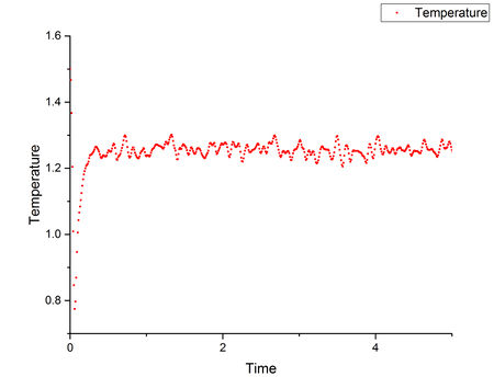
Plots of energy, temperature and pressure against time for 0.001 timestep are shown above. It can be seen that all the graphs reached equilibrium quickly at around T*=0.4 (the whole simulation ran for T*=100+ but the first T*=5 plots are shown here).Tick

A plot of energies at different timesteps against time.

From this plot, the energy simulation of 0.015 timestep did not converge which means 0.015 is too big for this simulation (bad choice). The other four timesteps all reached equilibrium. However, due to the relative large timesteps, timestep 0.01 and 0.0075 have higher average energy when equilibrium is reached. This is caused by the larger error in energy which results in a higher deviation from lowest energy. The 0.0025 and 0.001 timesteps have almost identical plots with less fluctuation than the other three plots which means they are both reliable timesteps. Therefore, 0.0025 is a good balance between time and accuracy (largest timestep to give acceptable results). Good

Running simulations under specific conditions

$E_K=\frac{3}{2}N{k}_{B}T$

$\frac{1}{2}\sum _i{m}_i{v}_i^2=\frac{3}{2}N{k}_{B}T(2)$

By imposing the desired tempreture, each velocity needs to be multiplied by coefficient $\gamma$,

$\frac{1}{2}\sum _i{m}_i(\gamma v_i{)}^2=\frac{3}{2}N{k}_B\mathfrak{𝔗}$

${\gamma }^2\frac{1}{2}\sum _i{m}_i{v}_i^2=\frac{3}{2}N{k}_B\mathfrak{𝔗}(3)$

divide (3) by (2) to get,

${\gamma }^2=\frac{\mathfrak{𝔗}}{T}$

$\gamma =\sqrt{\frac{\mathfrak{𝔗}}{T}}$ Tick

---

fix aves all ave/time 100 1000 100000 v_dens v_temp v_press v_dens2 v_temp2 v_press2

Fix ave/time command. The numbers 100, 1000 and 100000 denote that the average values are calculated every 100000 timesteps, the previous 1000 values, each 100 timesteps away, are used to calculate the average. For example, the values at timesteps 200100, 200200, 200300, ..., 300000 (1000 values in total) are used to calculate the average value on timestep 300000. Tick

---

A plot of simulated densities and ideal gas densities at different pressure against temperature.

As can be seen from this plot, both the simulated data and data from ideal gas law show a decrease in pressure when temperature increases in this NpT ensemble. NpT system tries to keep the pressure and temperature constant throughout the simulation. At higher temperature, the atoms have larger kinetic energy so higher repulsion between atoms is expected (higher pressure). In order to keep pressure constant while increasing temperature, the density must decrease which agrees with the trend in this plot.

The calculated ideal gas densities are higher than the simulated data at the same pressure. One of the fundamental approximation in ideal gas law is that particles do not interaction with each other, which means the atoms can get much closer, results in a higher density. The discrepancy increases with pressure. At higher pressure, the atoms repel each other more strongly while ideal gas law still treat the atoms the same. So a large discrepancy is expected. Good explanation

Calculating heat capacities using statistical physics

$C_V=\frac{\mathrm{V}\mathrm{a}\mathrm{r}\left[E\right]}{k_B{T}^2}=N^2\frac{{ϵ}^2\mathrm{V}\mathrm{a}\mathrm{r}\left[E^{*}\right]}{k_B\frac{{ϵ}^2}{{k_B}^2}{T^{*}}^2}=N^2\frac{k_B\mathrm{V}\mathrm{a}\mathrm{r}\left[E^{*}\right]}{{T^{*}}^2}$

Therefore, the heat capacity of the simulations can be calculated from its outputs. But the simulation boxes at different densities have different sizes. So it is more sensible to calculate the volumetric heat capacity ($\frac{C_V}{V}$）and compare.

$\frac{C_V}{V}=\frac{N^2}{{\sigma }^{3}V}\frac{k_B\mathrm{V}\mathrm{a}\mathrm{r}\left[E^{*}\right]}{{T^{*}}^2}$

The volumetric heat capacites at different temperature and densities are calculated and plotted below.

A plot of simulated volumetric heat capacity at different densities against temperature.

As can be seen from this plot, the volumetric heat capacities do not vary much when the temperature changes at each density. This is expected for a monoatomic system when there is no phase change.

The heat capacity increases when the density is increased, this is expected because there is more substance that can absorb thermal energy per volume.

An example input file can be found here. These heat capacity values look a little large. Heat capacity should decrease with increasing temperature for a monatomic crystal - think about the density of states and how it changes for larger temperatures

Structural properties and the radial distribution function

The radial distribution function (RDF) can be generated from the trajectory file and it illustrates the local environment in a particular structure.

A plot of g(r) of vapour, liquid and solid against r*.

As shown in this plot, the three phases have a very similar first peak at around r* = 1.1 which is close to the $r_{eq}$ calculated before. After the first peak, the vapour's g(r) immediately converges to 1; the liquid's g(r) fluctuates slightly then converges to 1; the solid's g(r) has a much greater fluctuation than the other two phases, then the fluctuation decreases but does not converge.

This shows that the gas has the most random distribution of atoms, ie. after the first peak caused by particle repulsions, the distribution of atoms around the centre appears to be uniform. The solid, on the other hand, shows a more structured distribution. This is expected as solid has the least degree of freedom and less subjected to random thermal motion. And the liquid's RDF shows a structure between vapour and solid. True but think about long range order

---

A plot of integral of g(r) of solid against r*.

The first three peaks are picked from the integral of g(r).

A fcc lattice.

The three closest neighbours in the fcc lattice are labelled in the figure. The difference in the g(r) integral peaks indicates the number of new lattice sites. The results are summarised below.

RDF results
Peak index (atom index)	Distance of lattice site from origin (lattice spacing)	coordination number
1	$\frac{\sqrt{2}}{2}$	12
2	$1$	6
3	$\frac{\sqrt{6}}{2}$	24

Since the second peak corresponds to the atom exactly 1 lattice spacing from the centre, lattice spacing = 1.53 (in reduced unit). So the lattice spacing is 5.21 Å. What's the coordination number for the solid?

Dynamical properties and the diffusion coefficient

$D=\frac{1}{6}\frac{\partial ⟨r^2\left(t\right)⟩}{\partial t}=\frac{1}{6}\frac{{\sigma }^2\partial ⟨{r^{*}}^2\left(t\right)⟩}{\sigma (m/ϵ{)}^{1/2}\partial t^{*}}$

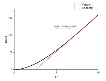
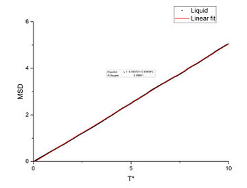
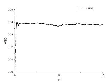
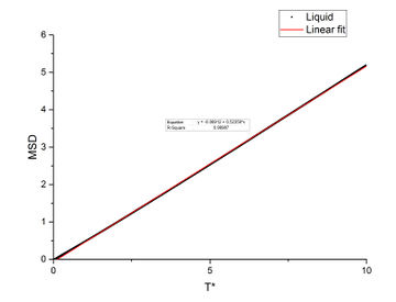
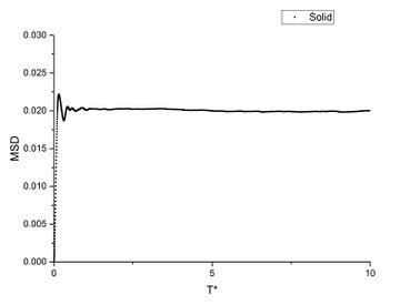
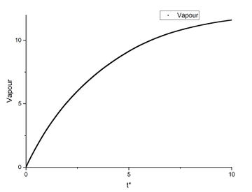
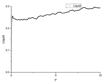
In order to find the diffusion coefficient, the mean square displacement of the system is monitored and plotted against T*. Best fit lines of the linear region are plotted as well and the gradients are found.

• Small system simulations
• 
• 
• 

• One million particles simulations
• 
• 
• 

From the gradients, the diffusion coefficients can be found as below.

Diffusion coefficient ($m^2{s}^{-1})$
	Small system	One million particles
Vapour	$1.88692\times 10^{-07}$	$1.67138\times 10^{-07}$
Liquid	$4.52269\times 10^{-09}$	$4.64877\times 10^{-09}$
Solid	$0$	$0$

The diffusion coefficients calculated from small system and large system have very close values. It can be seen that vapour has the largest diffusion coefficient and liquid diffuses slower than gas which is expected. Solid almost does not diffuse which is also expected.

Velocity Autocorrelation Function

The velocity of a 1-D harmonic oscillator is given by $v(t)=-\omega Asin(\omega t+\varphi )$,

and substitute this equation into the velocity autocorrelation function (VACF),

$\begin{array}{rl}C\left(\tau \right)& =\frac{\underset{-\mathrm{\infty }}{\overset{\mathrm{\infty }}{\int }}v\left(t\right)v(t+\tau )\mathrm{d}t}{\underset{-\mathrm{\infty }}{\overset{\mathrm{\infty }}{\int }}{v}^2\left(t\right)\mathrm{d}t}\\ C\left(\tau \right)& =\frac{\underset{-\mathrm{\infty }}{\overset{\mathrm{\infty }}{\int }}{\omega }^2{A}^{2}sin(\omega t+\varphi )sin(\omega t+\omega \tau +\varphi )\mathrm{d}t}{\underset{-\mathrm{\infty }}{\overset{\mathrm{\infty }}{\int }}{\omega }^2{A}^{2}si{n}^2(\omega t+\varphi )\mathrm{d}t}\\ C\left(\tau \right)& =\frac{\underset{-\mathrm{\infty }}{\overset{\mathrm{\infty }}{\int }}sin(\omega t+\varphi )sin(\omega t+\omega \tau +\varphi )\mathrm{d}t}{\underset{-\mathrm{\infty }}{\overset{\mathrm{\infty }}{\int }}si{n}^2(\omega t+\varphi )\mathrm{d}t}\end{array}$

By using angles addition formula,

$\begin{array}{rl}C\left(\tau \right)& =\frac{\underset{-\mathrm{\infty }}{\overset{\mathrm{\infty }}{\int }}sin(\omega t+\varphi )(sin(\omega t+\varphi )cos(\omega \tau )+sin(\omega t+\varphi )cos(\omega \tau ))\mathrm{d}t}{\underset{-\mathrm{\infty }}{\overset{\mathrm{\infty }}{\int }}si{n}^2(\omega t+\varphi )\mathrm{d}t}\\ C\left(\tau \right)& =\frac{\underset{-\mathrm{\infty }}{\overset{\mathrm{\infty }}{\int }}sin(\omega t+\varphi )(sin(\omega t+\varphi )cos(\omega \tau )+cos(\omega t+\varphi )sin(\omega \tau ))\mathrm{d}t}{\underset{-\mathrm{\infty }}{\overset{\mathrm{\infty }}{\int }}si{n}^2(\omega t+\varphi )\mathrm{d}t}\\ C\left(\tau \right)& =\frac{cos(\omega \tau )\underset{-\mathrm{\infty }}{\overset{\mathrm{\infty }}{\int }}si{n}^2(\omega t+\varphi )\mathrm{d}t+sin(\omega \tau )\underset{-\mathrm{\infty }}{\overset{\mathrm{\infty }}{\int }}sin(\omega t+\varphi )cos(\omega t+\varphi ))\mathrm{d}t}{\underset{-\mathrm{\infty }}{\overset{\mathrm{\infty }}{\int }}si{n}^2(\omega t+\varphi )\mathrm{d}t}\end{array}$

As $sin(\omega t+\varphi )cos(\omega t+\varphi )$ is an odd function, $\underset{-\mathrm{\infty }}{\overset{\mathrm{\infty }}{\int }}sin(\omega t+\varphi )cos(\omega t+\varphi ))\mathrm{d}t=0$

$\begin{array}{rl}C\left(\tau \right)& =\frac{cos(\omega \tau )\underset{-\mathrm{\infty }}{\overset{\mathrm{\infty }}{\int }}si{n}^2(\omega t+\varphi )\mathrm{d}t}{\underset{-\mathrm{\infty }}{\overset{\mathrm{\infty }}{\int }}si{n}^2(\omega t+\varphi )\mathrm{d}t}\\ C\left(\tau \right)& =cos(\omega \tau )\end{array}$ Good

A plot of VACF against timestep for harmonic oscilator, simulated liquid and solid.

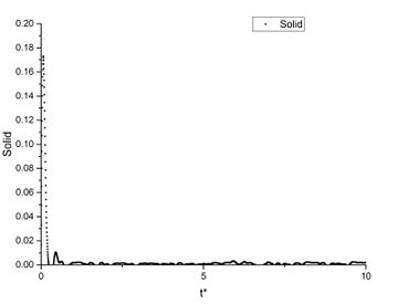
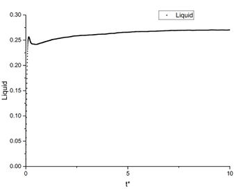
Minima in VACF of liquid and solid are the constant velocity points for the particles because the velocity correlation at that point does not change which means the velocity remains constant. Same as before, the liquid VACF decreases rapidly then converges to zero with only one minimum point. The solid VACF has several peaks before it converges to zero. This means liquid reaches random motion much quicker than solid which is expected as liquid is more flowable. In Velocity-Verlet algorithm and Lennard-Jones potential, the harmonic oscillator's velocity and position depend on its previous velocity. While in VACF, the velocity correlation with previous velocity is the subject of study. Good explanation

---

• Small system simulations
• 
• 
• 

• One million particles simulations
• 
• 
• 

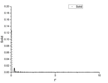
The plots with a larger system show smoother lines because of more particles are taken into the average. In particular, the integral of solid's VACF is almost 0. This can be explained by considering the solid structure of the fcc lattice. In the lattice, the atoms tend to vibrate in all directions rather than moving around, so the integral averages to nearly zero. As expected, the liquid's integral also converged much quicker than the vapour's integral and the vapour's integral may not fully converged yet.

The calculated diffusion coefficients are listed below.

Diffusion coefficient ($m^2{s}^{-1})$
	Small system	One million particles
Vapour	$2.06768\times 10^{-07}$	$1.74825\times 10^{-07}$
Liquid	$5.23594\times 10^{-09}$	$4.81884\times 10^{-09}$
Solid	$0$	$0$

These diffusion coefficients are similar to the previously calculated values from MSD. The largest source of error can be the simulation data. As can be seen in some of the figures, the simulation should be run long to ensure the value converges. When comparing to the provided data, the larger system shows less random fluctuation. So a larger system and longer simulation long will reduce error in this calculation. Good explanation