Talk:Mod:stmLS
JC: General comments: All tasks completed well with some good analysis of your results. Concentrate on making your answers as clear and focused as possible so that it is clear that you understand the material. Use left aligned text, rather than centred to make it easier to read.
Introduction to Molecular Dynamics Simulations
TASK: Open the file HO.xls. In it, the velocity-Verlet algorithm is used to model the behaviour of a classical harmonic oscillator. Complete the three columns "ANALYTICAL", "ERROR", and "ENERGY": "ANALYTICAL" should contain the value of the classical solution for the position at time , "ERROR" should contain the absolute difference between "ANALYTICAL" and the velocity-Verlet solution (i.e. ERROR should always be positive -- make sure you leave the half step rows blank!), and "ENERGY" should contain the total energy of the oscillator for the velocity-Verlet solution. Remember that the position of a classical harmonic oscillator is given by (the values of , , and are worked out for you in the sheet).
The values for the analytical column were calculated by using the harmonic oscillator motion equation...
To obtain the classical values for the energy, the following equation was utilised...
The following values were made available in the excel spreadsheet for the initial conditions
, , , , ,
Where
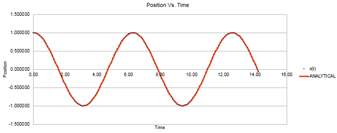
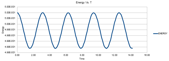
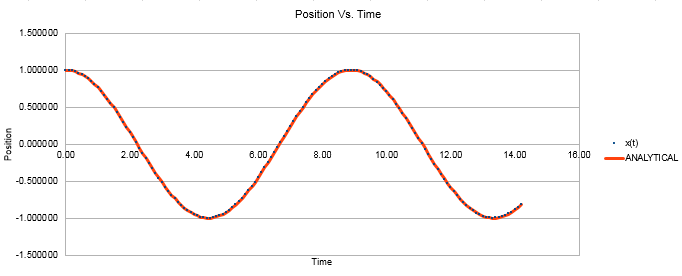
Figure 1 shows a plot of the velocity verlet algorithm, with position and time plotted. It can be seen from the overlap of the classical calculation and the velocity verlet line that the two methods are in good agreement.
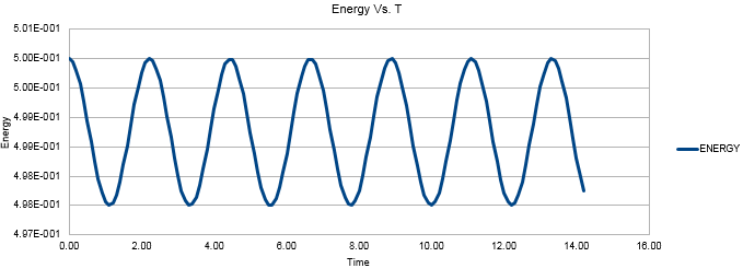
Figure 2 shows the Energy value oscillating between roughly 4.988 and 0.5000. As we are dealing with the quantum harmonic oscillator, in an ideal situation the sum of the potential and kinetic energy of the system will be constant as no energy is being lost to the surroundings. This results in infinite perpetual vibrations as the system extends and compresses whilst exchanging its forms of energy between potential and kinetic. The time average of the energy transpires to be essentially constant. There are oscillations of very small amplitude (approximately 0.125% of the average value) around the average value which follow sinusoidal behavior. 0.125% oscillations around the average value can be considered to agree with the expected physical behavior of our system.
JC: We are simulating the classical harmonic oscillator, not the quantum one.
The initial conditions for the mass were varied to observe the effect it would have. The initial conditions were changed to the following values...
, , , , ,
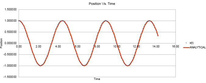
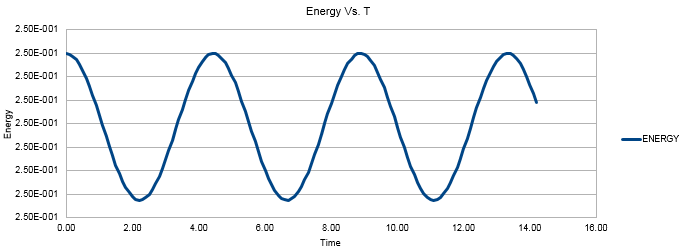
Decreasing the mass of the system increased the frequency of the oscillations in the position and energy vs. time graphs. This can be rationalised by looking at the equation relating the frequency of the oscillations to the mass of the system. (Equation 3) This equation can also be used to make sense of the change in the graphical plots when the force constant, k, is changed. Figures 5 and 6 both show the directly proportional effects on the frequency of decreasing k from 1 to 0.5 whilst the mass reverts to being 1.
TASK: For the default timestep value, 0.1, estimate the positions of the maxima in the ERROR column as a function of time. Make a plot showing these values as a function of time, and fit an appropriate function to the data.
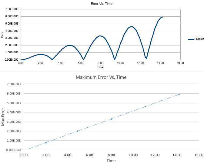
The second column in the spreadsheet was the Error column. This column was calculated by taking the difference between the analytical value obtained and the velocity verlet value. Figure 7 shows that the values in question are very small, however they increase in magnitude with time due to the the velocity verlot algorithm incorporating the Taylor expansion which causes small errors to build up over time. Figure 7 also shows a fit of an appropriate function to the error vs time data. This gives a straight line with equation y = 0.0004x - (7E-05).
TASK: Experiment with different values of the timestep. What sort of a timestep do you need to use to ensure that the total energy does not change by more than 1% over the course of your "simulation"? Why do you think it is important to monitor the total energy of a physical system when modelling its behaviour numerically?
In order for the total energy of the system to stay within 1% of the average value, it is important that a short timestep is used. Large timesteps result in large fluctuations of energy with greater standard deviation values. This also ensures our model corresponds to a thermodynamically closed system that obeys the law of conservation of energy. The upper timestep limit has been found to be 0.21s in order for the energy to remain between the values of 0.4944 and 0.5040.
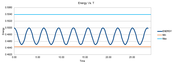
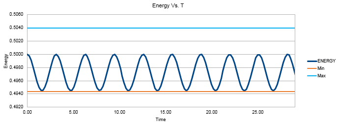
JC: Good analysis and choice of timestep.
TASK: For a single Lennard-Jones interaction, , find the separation, , at which the potential energy is zero. What is the force at this separation? Find the equilibrium separation, , and work out the well depth (). Evaluate the integrals , , and when .
In order to find the seperation at which the potential energy , we can substitute the following terms into the Lennard-Jones interaction equation...
Thus giving us...
Dividing through by 4 epsilon, rearranging the equation and cancelling out the indices yields...
As the force acting on a body is given by
we must differentiate the equation for the potential. This gives us...
Which simplifies out to
The equilibrium separation is the separation for which
Therefore when F=0 and
We can now evaluate the well depth by substituting the solution for into the Lennard-Jones equation
Evaluation of the integrals with the following parameters gives...
TASK: Estimate the number of water molecules in 1ml of water under standard conditions. Estimate the volume of water molecules under standard conditions.
This task has been completed by considering the density of water to find the mass of water in 1 mL. Dividing the mass in grams by the molecular mass will yield the number of moles in 1mL. Multiplying the number of moles by Avogadro's number will tell us the number of molecules in 1mL of water. The units used throughout these calculations were ensured to be homogenous.
Taking the Molecular mass of water as 18.015 g/mol gives 0.0555 moles. Multiplying this value by Avogadro's number gives
molecules in 1mL of water under standard thermodynamic conditions.
We can also work out the volume taken up by 10000 molecules of water by employing the same relations as used above.
Thus, as N=10,000
Once again using 18.015 g/mol as the molecular mass of water gives us...
Using the same value of density as used above gives...
TASK: Consider an atom at position in a cubic simulation box which runs from to . In a single timestep, it moves along the vector . At what point does it end up, after the periodic boundary conditions have been applied?
If we were to ignore the periodic boundary conditions, the final position of the atom would be the sum of the vectors and , which is . The periodic boundary conditions used means that the atoms final position will be
TASK: The Lennard-Jones parameters for argon are . If the LJ cutoff is , what is it in real units? What is the well depth in ? What is the reduced temperature in real units?
As and the Lennard-Jones cutoff distance is 1.09nm.
The well depth is given by
Finally, the reduced temperature has also been calculated in real units
JC: All maths and calculations correct and clearly laid out. Make sure that you give answers to the same number of significant figures as in the question.
Equilibration
TASK: Why do you think giving atoms random starting coordinates causes problems in simulations? Hint: what happens if two atoms happen to be generated close together?
If we were to assign random starting coordinates to our liquid simulation and the size of our simulation box relative to the number of atoms we are simulating is small, there is a high likelihood of atoms being generated in very close proximity to one another. From the Lennard-Jones potential equation, we know that the term describes Pauli repulsion at short ranges due to overlapping electron orbitals thus placing atoms close to one another will lead to unrealistically high energy potentials, which will result in large forces and accelerations applied to the atoms to lose their potential energy by moving at very high speeds. This will mean we will have to use particularly small timesteps in order to attain accurate results. In this experiment we get around this problem by placing the atoms on lattice points of a simple cubic lattice in the hope that the atoms arrange themselves into a more realistic configuration over time.
It should be remembered that the LJ potential is a classical approximation that is favored in computational chemistry due to it's simplicity. More complex ab initio methods describe the interaction of molecules with one another more accurately.
JC: Good explanation.
TASK: Satisfy yourself that this lattice spacing corresponds to a number density of lattice points of . Consider instead a face-centred cubic lattice with a lattice point number density of 1.2. What is the side length of the cubic unit cell?
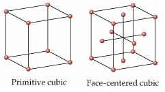
Our lattice spacing is given by
Lattice spacing in x,y,z = 1.07722 1.07722 1.07722
Hence, the volume of the unit cell is given by
Therefore
When considering a face centred cubic (FCC) lattice, we must remember that there are four atoms within the unit cell. Hence and which gives
TASK: Consider again the face-centred cubic lattice from the previous task. How many atoms would be created by the create_atoms command if you had defined that lattice instead?
 region box block 0 10 0 10 0 10
create_box 1 box
These lines from the input file create a 10 x 10 x 10 array of unit cells. As there are 1000 unit cells, and an FCC lattice has 4 atoms per unit cell, we would have a total of 1000 atoms crated by the create_atoms command.
If the FCC lattice (which has 4 atoms per unit cell) were used, the create_atoms command would yield a total of 4000 atoms.
TASK: Using the LAMMPS manual, find the purpose of the following commands in the input script:
mass 1 1.0
pair_style lj/cut 3.0
pair_coeff * * 1.0 1.0
The first line of the above input file "mass 1 1.0" defines the mass of the atoms being simulated to 1.0. Using an asterisk to replace the number after "mass" would result in all atoms in the simulation being assigned identical masses. Alternatively, an asterisk can also be placed before the specified number in which case all the atom types from 1 to the specified number will be assigned as the same mass. The asterisk may also be placed after the number to signify that all atoms after that number are to be given the same specified value for the mass.
The middle line of the command calculates the Lennard Jones (LJ) potential between the pairs of atoms. Note that the cutoff value (3.0) gives the distance in reduced units at which the LJ interactions will be calculated up until. As the LJ potential converges towards zero at large values of r, it is useful to have a cutoff distance in order to decrease computational cost of calculations.
The final line of the command specifies the pairwise force field coefficients. In LAMMPS, pairwise force fields account for many body interactions. They are still classified as “pairwise” potentials because the set of interacting atoms changes with time (unlike molecular bonds) and thus a neighbor list is used to find nearby interacting atoms. The asterisk once again signifies that this applies to all atom types present in the box. (In our example we only have one type of atom present).
JC: Why don't we need to use an asterisk in the mass command, what does the first arguement of the mass command specify? For a Lennard-Jones potential, the pairwise coefficients are sigma and epsilon.
TASK: Given that we are specifying and , which integration algorithm are we going to use?
The velocity-verlet algorithm would be ideal for this scenario as it is a requirement for and to be defined as such before any simulation is run.
TASK: Look at the lines below.
### SPECIFY TIMESTEP ###
variable timestep equal 0.001
variable n_steps equal floor(100/${timestep})
variable n_steps equal floor(100/0.001)
timestep ${timestep}
timestep 0.001

### RUN SIMULATION ###
run ${n_steps}
run 100000
The second line (starting "variable timestep...") tells LAMMPS that if it encounters the text ${timestep} on a subsequent line, it should replace it by the value given. In this case, the value ${timestep} is always replaced by 0.001. In light of this, what do you think the purpose of these lines is? Why not just write:
timestep 0.001
run 100000
The reason we employ the code which incorporates variable timestep is that it means that we can change the timestep and still ensure that the total simulation time remains constant. This is achieved by changing the number of timesteps in accordance with modifying the timestep duration. In the simplified version of the code, doubling the duration of the timestep would also double the total simulation time. This allows for more meaningful comparisons to be made.
TASK: make plots of the energy, temperature, and pressure, against time for the 0.001 timestep experiment (attach a picture to your report). Does the simulation reach equilibrium? How long does this take? When you have done this, make a single plot which shows the energy versus time for all of the timesteps (again, attach a picture to your report). Choosing a timestep is a balancing act: the shorter the timestep, the more accurately the results of your simulation will reflect the physical reality; short timesteps, however, mean that the same number of simulation steps cover a shorter amount of actual time, and this is very unhelpful if the process you want to study requires observation over a long time. Of the five timesteps that you used, which is the largest to give acceptable results? Which one of the five is a particularly bad choice? Why?
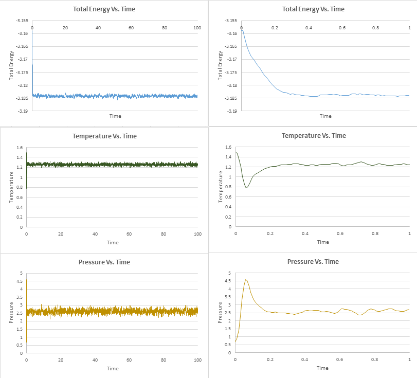
The time axis of the graphs on the left were adjusted to a smaller scale so that it is possible to tell more accurately when the system has reached equilibrium. We deem the system to have reached equilibrium when the time average of the property in question fluctuates around a constant value. This appears to occur at different times for the different thermodynamic parameters, so we will take the highest value of time to be the time at which the system has reached equilibrium. This transpires to be the energy which reaches equilibrium at around t=0.3.
JC: Good idea to look at equilibration time.

From the first plot shown in Figure 12, it can be seen which of the timesteps employed leads to better results. It is evident that the timestep where t=0.015 has not reached equilibrium, hence this timestep would constitute a particularly bad choice. In order to distinguish between which of the other timesteps leads to better results, the second plot shows a zoomed in region of the energy vs. time plots of the different timesteps. It can be seen that the main difference between the different timesteps lies in how much they oscillate around an average energy value. Smaller oscillations are deemed to indicate that the energy readings are more accurate. t=0.001 and t=0.0025 are the two best timesteps to use in terms of the average energy value attained. The computational cost of using the 0.0025 timestep would be less than half that of the 0.001 timestep and the accuracy of the energy values attained are comparable, hence t=0.0025 would be an ideal choice of timestep.
JC: Should the average total energy depend on the timestep used? Timesteps of 0.001 and 0.0025 both give the same average energy.
Running Simulations Under Specific Conditions
TASK: Choose 5 temperatures (above the critical temperature ), and two pressures (you can get a good idea of what a reasonable pressure is in Lennard-Jones units by looking at the average pressure of your simulations from the last section). This gives ten phase points — five temperatures at each pressure. Create 10 copies of npt.in, and modify each to run a simulation at one of your chosen points. You should be able to use the results of the previous section to choose a timestep. Submit these ten jobs to the HPC portal. While you wait for them to finish, you should read the next section.
Due to the findings of the last task, we have chosen the timestep of 0.0025 for the calculations as it provides a good compromise between accuracy of data and computational cost. The 5 temperatures chosen were all in 1 reduced T increments above the critical temperature (1.5-5.5T). 3 pressures (2.5, 3.0 and 3.5) were chosen instead of 2 in order to see if the trend upon increasing pressure is linear or follows a different trend.
TASK: We need to choose so that the temperature is correct if we multiply every velocity . We can write two equations:
Solve these to determine .
These equations can be solved for by adding the equations together, substituting in and factorising as shown below...
JC: Correct.
TASK: Use the manual page to find out the importance of the three numbers 100 1000 100000. How often will values of the temperature, etc., be sampled for the average? How many measurements contribute to the average? Looking to the following line, how much time will you simulate?
 fix aves all ave/time 100 1000 100000 v_dens v_temp v_press v_dens2 v_temp2 v_press2
run 100000
The different thermodynamic properties being simulated are computed by the fix command which tells us the average for any of the given variables. The numbers that follow the command (100 1000 100000) give some parameters which define how the average will be taken. The number 100 is the Nevery and instructs LAMMPS to take a sample every 100 timesteps. The number 1000 is the NRepeat which tells LAMMPS how many samples are used to calculate the final average value. Finally, the 100000 is the NFreq number and average thermodynamic quantities will be calculated at timesteps of multiples of this value. As the timestep has been defined as 0.0025, a simulation of 100000 data points yields 250 reduced time unit simulations.
TASK: When your simulations have finished, download the log files as before. At the end of the log file, LAMMPS will output the values and errors for the pressure, temperature, and density . Use software of your choice to plot the density as a function of temperature for both of the pressures that you simulated. Your graph(s) should include error bars in both the x and y directions. You should also include a line corresponding to the density predicted by the ideal gas law at that pressure. Is your simulated density lower or higher? Justify this. Does the discrepancy increase or decrease with pressure?
The ideal gas law can be rearranged from into in order to give us the number density. Note also that in this expression when calculations are being performed in reduced units. Thus simplifying the equation to . The figure below shows a plot of number density vs. temperature for the various conditions employed. Note that error bars for the standard error in the computed density values have not been included as the standard error is around 0.005-0.008% which would be difficult to observe when plotted. The error bars for the temperature in reduced units have been included. It can be seen that as the temperature is increased, the standard error increases.
It can be clearly seen from the graph produced that the densities of the simulated data points are all lower than their counterparts calculated using the ideal gas law. This can be explained by the fact that the ideal gas equation makes a series of assumptions such as the distance between molecules being much larger than the size of the molecules and that there are no intermolecular forces between the molecules. These assumptions are not made in the liquid simulation that has been run which uses the Lennard Jones interactions that incorporates short range repulsive terms due to overlapping electron orbitals, hence the atoms in the liquid simulation will be found at a greater separation which explains the lower density in these calculations.
The discrepancy between the simulated data and the data calculated using the ideal gas law increases with pressure. The reasoning for this is similar to that which has been explained above. At high pressures, liquid particles are pushed together more and hence repel more strongly whereas this repulsion is not accounted for in the ideal gas law. As pressure increases, the assumption that there are no intermolecular forces between the gas particles may hold true at low pressures, but certainly not at high pressures.
Finally, it can also be seen that increasing the temperature causes the sets of data obtained by simulation and the ideal gas law to converge. This can be explained by there being greater kinetic energy within each molecule at higher temperatures. This energy predominates and means that intermolecular repulsions become increasingly negligible and the ideal gas law description starts to fit better.
It would be interesting to see how well the Van der Waals equation given above (which takes into account intermolecular forces and models elastic collisions between hard spheres) agrees with the liquid simulation data. Note that the Van der Waals equation does not work particularly well near the transition between gas and liquid. The Maxwell equal area rule given below models liquid vapour phase boundaries more accurately.
JC: Good explanation and good suggestion to try the Van der Waals equation instead.
Calculating Heat Capacities Using Statistical Physics
TASK: As in the last section, you need to run simulations at ten phase points. In this section, we will be in density-temperature phase space, rather than pressure-temperature phase space. The two densities required at and , and the temperature range is . Plot as a function of temperature, where is the volume of the simulation cell, for both of your densities (on the same graph). Is the trend the one you would expect? Attach an example of one of your input scripts to your report.
One of the input scripts used to complete the task of finding the heat capacity at T=2.2 and d=0.2 has been included below.
### DEFINE SIMULATION BOX GEOMETRY ###

variable d equal 0.2
lattice sc ${d}
region box block 0 15 0 15 0 15
create_box 1 box
create_atoms 1 box

### DEFINE PHYSICAL PROPERTIES OF ATOMS ###
mass 1 1.0
pair_style lj/cut/opt 3.0
pair_coeff 1 1 1.0 1.0
neighbor 2.0 bin

### SPECIFY THE REQUIRED THERMODYNAMIC STATE ###
variable T equal 2.2
variable timestep equal 0.0025

### ASSIGN ATOMIC VELOCITIES ###
velocity all create ${T} 12345 dist gaussian rot yes mom yes

### SPECIFY ENSEMBLE ###
timestep ${timestep}
fix nve all nve

### THERMODYNAMIC OUTPUT CONTROL ###
thermo_style custom time etotal temp press
thermo 10

### RECORD TRAJECTORY ###
dump traj all custom 1000 output-1 id x y z

### SPECIFY TIMESTEP ###

### RUN SIMULATION TO MELT CRYSTAL ###
run 10000
unfix nve
reset_timestep 0

### BRING SYSTEM TO REQUIRED STATE ###
variable tdamp equal ${timestep}*100
fix nvt all nvt temp ${T} ${T} ${tdamp}
run 10000
reset_timestep 0

### MEASURE SYSTEM STATE ###
thermo_style custom step etotal temp
variable etot equal etotal
variable etot2 equal etotal*etotal
variable temp equal temp
fix aves all ave/time 100 1000 100000 v_temp v_etot v_etot2
unfix nvt
fix nve all nve
run 100000

variable avetemp equal f_aves[1]
variable avetemp2 equal f_aves[1]*f_aves[1]
variable e2bracket equal f_aves[3]
variable ebracket2 equal f_aves[2]*f_aves[2]
variable cv equal atoms*atoms*(${e2bracket}-${ebracket2})/${avetemp2}
variable volume equal vol
variable cvv equal ${cv}/${volume}

print "Averages"
print "--------"
print "Density: ${density}"
print "AveTemperature: ${avetemp}"
print "HeatCapacity: ${cv}"
print "Volume: ${volume}"
print "HeatCapacityOverVolume: ${cvv}"
Statistical thermodynamics tells us that given parameters tend to fluctuate about an average value which is considered to be the equilibrium value. These fluctuations help us to deduce the heat capacity of the system under study.
The fluctuation itself is given by the variance term in the equation above. As the variance is itself a function of the number of molecules , we can deduce that a larger system in our computation will yield a more accurate average value for a given parameter such as energy.
It would be expected for the Isochoric heat capacity (which is an extensive property) to increase with density at any given temperature as a denser system at constant volume will contain more particles which requires proportionally greater amounts of energy to raise the temperature of. This trend has been confirmed by the figure above.
Another interesting observation that has been made is that the isochoric heat capacity decreases as the temperature increases. This trend is perhaps arising from the fact that at higher temperatures the density of states is greater, this means there are a greater number of accessible energy levels for a particular temperature and less energy needs to be provided to proportionally populate these energy levels. Hence, the overall transfer of heat to the system becomes more facile.
JC: Your plot has been replaced by another image, but the explanations for the trends that you see are good.
Structural Properties and the Radial Distribution Function
TASK: perform simulations of the Lennard-Jones system in the three phases. When each is complete, download the trajectory and calculate and . Plot the RDFs for the three systems on the same axes, and attach a copy to your report. Discuss qualitatively the differences between the three RDFs, and what this tells you about the structure of the system in each phase. In the solid case, illustrate which lattice sites the first three peaks correspond to. What is the lattice spacing? What is the coordination number for each of the first three peaks?
The phase diagram for the Lennard-Jones system was used to select the temperature and pressures for each of the systems. RDF's were then calculated from the trajectory files obtained.
Gas - Density = 0.05 - Temperature = 1.2
Liquid - Density = 0.8 - Temperature = 1.2
Solid - Density = 1.2 - Temperature = 1.2
The radial distribution function (RDF) describes how the density of particles varies as a function of distance from a defined reference particle. Analysis of the RDF provides an insight into the relative arrangement and the degree of order within each of the different states that have been analysed. It is possible to compare simulated RDF's to experimental RDF's which have been derived using X-ray diffraction.
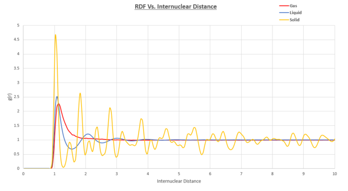
Something that the RDF's of all three phases have in common is the fact that the value for the RDF at internuclear distances of less than approximately 0.9 equates to zero. This can be explained by the short range Lennard Jones repulsion term which is raised to the power of 12 and as such particles are prevented from being in such close proximity to one another.
Notice that within the gas phase RDF, we only observe one broad peak at an internuclear distance of approximately 1. Other than this, the RDF is featureless suggesting a lack of any intrinsic order within the system.
For the liquid RDF, we observe three main peaks. The amplitude of the peaks decreases with internuclear distance. The rapid random brownian motion within a liquid coupled with a lack of any long range order makes it hard to describe the order within a liquid. We can make sense of the RDF by taking an instantaneous snapshot of the liquid in 2D. It can be seen from Figure 13 that in relation to the central molecule, there are layers of molecules surrounding the central one with the higher coordination shells being more diffuse and less ordered than the first. This reduction in order explains the decreasing amplitude in the liquid RDF. At short internuclear distances, there are striking similarities between the RDF of a crystalline solid and the RDF of a liquid however the RDF decays to a constant value at large distances. From the RDF, other thermodynamic parameters such as the total energy of the system can be studied. This is done by considering the volume of a coordination sphere in 3D which contains particles and multiplying this term by the pair potential at a given distance. You then integrate with respect to r between 0 and and multiply the results by N/2 to ensure that each interaction is only counted once. The end result of this is
For the solid, the atoms are located in the lattice sites of a Face Centered Cubic (FCC) lattice. We can interpret the peaks as indicating a particularly favored separation distance. As there are peaks throughout the entirety of the internuclear distance range we are observing we can deduce that there is long range order within our solid system. Notice also how the peaks are much narrower than those observed for the liquid or gaseous RDFs which is an indication that there is less random atomic motion present in the solid. Performing the RDF at 0K with a perfectly crystalline solid with no defects should turn the peaks into extremely thin lines as the thermal motion will be minimised.
JC: Good description of the RDF and structure for the different phases.
In order to ascertain which lattice sites correspond to the first three peaks in the RDF we must look more closely at the structure of a single unit cell. It would make sense for the 3 peaks to correspond to the smallest 3 interatomic distances. These distances have been highlighted in the figure below.
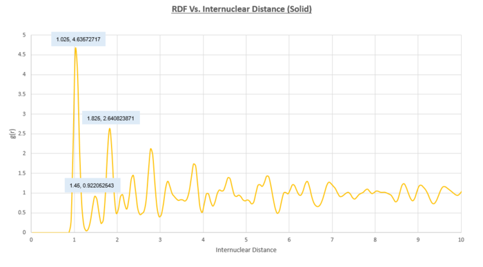
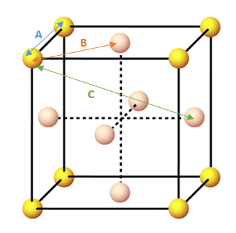
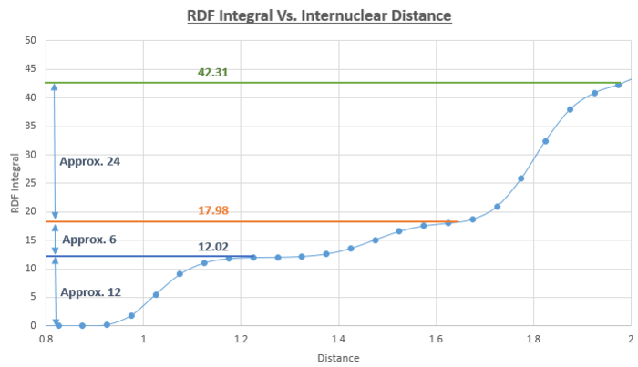
By reading off the graph of the solid RDF, we can say that the second peak which represents the length of the unit cell occurs at an interatomic distance of 1.45. We also know that the distances of 1.025 and 1.825 correspond to the other two distances highlighted in the figure above. From this diagram we can also deduce the coordination number of the first three peaks on the RDF as being 12, 6 and 24. An additional way of confirming this observation is to plot a continual integral along the distance axis of the solid RDF and take the differences between the regions where the integral plateaus out.
JC: You could have calculated the lattice parameter from the first and third peaks as well and averaged them to get a more accurate value for the lattice parameter.
Dynamical Properties and the Diffusion Coefficient
TASK: In the D subfolder, there is a file liq.in that will run a simulation at specified density and temperature to calculate the mean squared displacement and velocity autocorrelation function of your system. Run one of these simulations for a vapour, liquid, and solid. You have also been given some simulated data from much larger systems (approximately one million atoms). You will need these files later.
The densities used to run the simulations for the gas, liquid and solid were 0.05, 0.8 and 1.2 respectively.
TASK: make a plot for each of your simulations (solid, liquid, and gas), showing the mean squared displacement (the "total" MSD) as a function of timestep. Are these as you would expect? Estimate in each case. Be careful with the units! Repeat this procedure for the MSD data that you were given from the one million atom simulations.
The diffusion coefficient for a system at equilibrium is given by
As the timestep in use is 0.002 time units, we divide the gradient of the graph by this value to convert timestep units into time units before multiplying by 1/6 to yield the diffusion coefficient with the correct units.

As we must find the gradient of the line in order to obtain a value for the diffusion coefficient, it is essential our value for the gradient is as accurate as possible in order to prevent the propagation of any errors. Unfortunately, the initial timesteps of the vapour system did not follow a linear pattern and thus deviates to a considerable extent from the line of best fit drawn. This is confirmed by the R squared value of 0.9807. A more linear fit for the line can be found if we were to only consider timestep values above 2000. When this has been done, the R squared value increases to 0.9973.
We can explain the deviation from linearity at low timestep values by considering the distances between gaseous atoms. At low timesteps, gaseous atoms will be far away from one another and will not be undergoing collisions with one another. This means that the atoms move with a constant velocity, with distance being directly proportional to time. As mean square displacement is given by
Initially, the graph follows a parabolic relationship at an area called the Ballistic regime. This is because the gaseous atoms are positioned randomly at a large distance from one-another. This means there are not as many collisions between the gaseous atoms as would be expected and brownian motion is not observed as the atoms will move at a constant velocity. If the atoms are moving with a constant velocity, it can be deduced from the MSD equation that the line will be parabolic as the MSD is proportional to the square of time.
JC: This explanation is correct, but the writing is quite repetitive and not very clear. Try to make it more focused and concise.
Once the line turns linear at around 1500 timesteps the motion of the atoms can be described by brownian motion. Hence, the diffusion coefficient is given by
JC: Is the graph really linear at 1500? Plot the line of best fit that you used to calculate the diffusion coefficient on your graph.
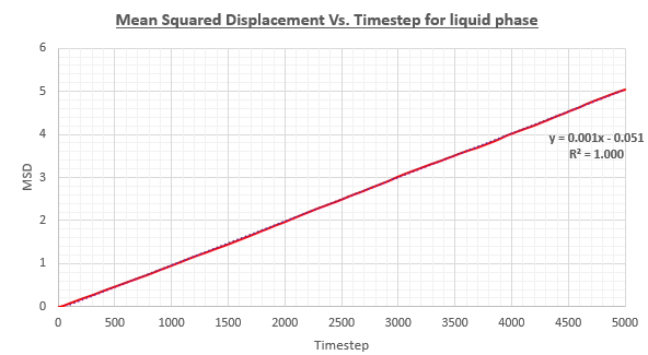
As the atoms within a liquid are already initially in close contact with one another, no non linear relationship is initially seen as brownian motion is in play at all times due to the close proximity of the atoms to one another. The diffusion coefficient has once again been calculated
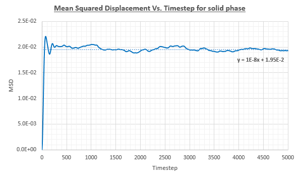
The plot for the MSD Vs. Timestep was considerably different for the solid phase in comparison to the liquid and vapour phases. In the liquid and vapour phases the MSD increased throughout the simulation. In contrast, the solid shows an initial sharp increase from 0 to around 0.02 after which point the the MSD remained roughly constant. This can be rationalised by the fact that in a solid, atoms are generally more tightly bound to their lattice sites. The diffusion coefficient was found by only considering the gradient of the line after the MSD had reached a roughly constant value.
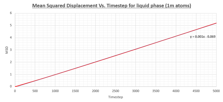
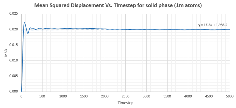
The simulations were also run on a system with one million atoms as can be seen in the figures below. The diffusion coefficients were figured out as shown above and a comparison table is also provided below.

| Diffusion coefficient (smaller system) | Diffusion coefficient (1 million atom system) | |
|---|---|---|
| Vapour Phase | 2.942 | 2.933 |
| Liquid Phase | 0.083 | 0.083 |
| Solid Phase | 8.33*10^{-7} | 8.33*10^{-7} |
The table above shows that the obtained values for the diffusion coefficient are in good agreement between the smaller system and the system with 1 million atoms. Therefore, it would make sense to reduce the computational cost of the calculation by performing the simulation on a smaller system. A more notable difference can be observed in the gradient of the solid phase MSD Vs. Timestep graph which remains at a more constant value throughout the simulation.
JC: Did you use the lines of best fit on these graphs to calculate the diffusion coefficients or did you use a line fitted to only the linear part of the graph? Does the solid graph really stay more constant or is it just that the y axis scale is different?
TASK: In the theoretical section at the beginning, the equation for the evolution of the position of a 1D harmonic oscillator as a function of time was given. Using this, evaluate the normalised velocity autocorrelation function for a 1D harmonic oscillator (it is analytic!):
In order to evaluate the above expression, the functions inside the integral must be expressed explicitly. This can be achieved by differentiating the following equation for the classical harmonic oscillator as we know that the differential of a displacement function yields a velocity function...
This function can be differentiated using the chain rule bu making the substitution into the above formula.
Substituting these terms into the general formula for the chain rule gives
We also have the term in the expression we must evaluate. We can differentiate the harmonic oscillator equation using the same method as above for when to give us
We can now rewrite the equation we must evaluate and plug in the values for and
The terms can be cancelled throughout the expression to give
The next stage involves using the following trigonometric identity to help simplify the formula
This can be applied to our expression by stating that and
Therefore
Inputting this trigonometric identity into gives us
Expanding the brackets in the numerator and subsequent separation of the integral into two integrals using the following relation
Gives
As the differential is being performed with respect to t, we can remove the terms containing Tau. Namely and . Removing these terms and simplifying by cancelling out like terms leads us to
Notice how the left hand side of our function contains an even symmetrical function as well as an unsymmetrical odd function which are being multiplied together. This results in an odd function which integrates to a value of 0. If the denominator turns out to be non zero, we can ignore the entirety of the first term. If the denominator is zero, the term becomes undefined as we would be dividing by zero.
Therefore, we can simplify the equation to
JC: Good, clear derivation.
Be sure to show your working in your writeup. On the same graph, with x range 0 to 500, plot with and the VACFs from your liquid and solid simulations. What do the minima in the VACFs for the liquid and solid system represent? Discuss the origin of the differences between the liquid and solid VACFs. The harmonic oscillator VACF is very different to the Lennard Jones solid and liquid. Why is this? Attach a copy of your plot to your writeup.
The Velocity Autocorrelation Function (VACF) is a time dependant statistical correlation between two variables at different points in time which can help us understand the microscopic processes at play in our molecular systems. It works by taking into account the velocity in the x,y and z directions at a chosen point in time for our system.
From this, we can calculate the first value of the VACF when t=0 by taking an average of the scalar products over all the atoms being considered in the system.
The velocity at the next timestep is then calculated
Inputting different timesteps allows us to obtain a plot for the VAF
Which can be denoted as
These are the steps that have been undertaken to produce the following plot
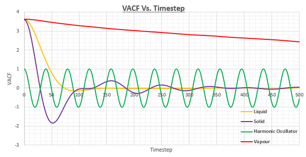
It can be seen that all of the plots start at a maximum point when . This can be rationalised as it means that .
The minima within the VACF plots correspond to a change in the direction of the atoms due to a collision. At the minima, it can be said that the difference between and is at a maximum.
The VACF for the vapour system has also been included in figure 26. It can be seen that there is a significant discrepancy between the vapour system in comparison to the other systems. This can be rationalised by the gaseous atoms 'forgetting' or decorrelating with their initial velocity due to the presence of weak forces.
When the interatomic forces are more notable, as is the case with liquids and solids which have much higher densities, the atoms will seek to minimise their potential energy by locating a coordinate where repulsive and attractive forces reach an energetically favourable compromise. These locations are more fixed for solids than for liquids which leads to oscillations. We would therefore expect to see the VACF reverse in the plot for the solid phase, and this is indeed the case. The oscillations can be seen to have differing amplitudes which shows a steady decay with time until the VACF plot becomes almost horizontal implying only very weak forces are left acting on the system. The reason the plot becomes horizontal rather than continuously oscillating is that perturbative damping forces disrupt perfect harmonic oscillator motion.
As there are no collisions in the harmonic oscillator, the VACF fluctuates around the same value over the course of the simulation suggesting that the velocity never decorrelates.
Liquids can be considered to behave in a similar manner to solids in some aspects, however the atoms do not have fixed regular positions as we saw by studying the mean square displacement of their atoms in the previous section. The higher diffusion coefficients present within liquids do not allow for any oscillatory motion to be seen, which is confirmed by the VACF plot only having one minimum point as the result of atoms colliding with their solvent cage. Instead of being considered as a damped harmonic oscillator, it is more accurate to say that it is essentially a collision between atoms which then proceed to diffuse away from one another.
JC: Collisions cause the VACF to decorrelate as atom motion becomes more randomised.
As well as allowing us to infer the above, the VACF can be fourier transformed to give interesting information about the frequencies of the molecular processes at play which can help us rationalise Infrared spectra. The VACF is also related to Mean Square Displacement using Green-Kubo relations, meaning we can acquire diffusion coefficients for our system.
TASK: Use the trapezium rule to approximate the integral under the velocity autocorrelation function for the solid, liquid, and gas, and use these values to estimate in each case. You should make a plot of the running integral in each case. Are they as you expect? Repeat this procedure for the VACF data that you were given from the one million atom simulations. What do you think is the largest source of error in your estimates of D from the VACF?


| Diffusion coefficient (smaller system) | Diffusion coefficient (1 million atom system) | |
|---|---|---|
| Vapour Phase | 3.294 | 3.268 |
| Liquid Phase | 0.098 | 0.090 |
| Solid Phase | 1.84 x 10⁻⁴ | 4.53 x 10⁻⁵ |
The diffusion coefficients in the table above have been calculated from the VACF running integral. As was the case when the diffusion coefficient (D) was calculated using the Mean Square Displacement method the vapour has the highest D value, followed by the liquid and then the solid. The values obtained using the two different methods are within the same orders of magnitude but show a significant discrepancy. I would be more inclined to think that the MSD method would yield more accurate values as the VACF running integral method uses the trapezium rule which has limited efficacy. Another problem is that the VACF method will be more accurate if we integrate to infinite time, however this cause the VACF to accumulate a great deal of noise. More accurate values of D and other transport properties can be found by using more sophisticated integration methods such as Gaussian quadrature which uses a weighted sum of function values at specific points within the integration domain.
As with the MSD method, it seems unnecessary to run the simulation on 1 million atoms as the increase in accuracy would not be worth the additional computational cost of the calculation.
JC: Good comparison, what are the units for the diffusion coefficient?
| You have been marking this page since 13:46 Tuesday, April 21, 2026 . |
