Talk:Mod:ss11012cmp

Introduction to the Ising Model

TASK 1 - Show that the lowest possible energy for the Ising model is $E = - D N J$ , where $D$ is the number of dimensions and $N$ is the total number of spins. What is the multiplicity of this state? Calculate its entropy.

The Interaction energy, E, is given by

E = - \frac{1}{2} J \sum_{i}^{N} \sum_{j \in n e i g h b o u r s (i)} s_{i} s_{j}

Each spin in an Ising lattice of D dimensions, has 2*D adjacent interactions. In the lowest possible energy configuration parallel alignment of adjacent spins is required, this makes all spins aligned with respect to any neighbour cells.

From this we obtain

\sum_{i}^{N} \sum_{j \in n e i g h b o u r s (i)} s_{i} s_{j} = 2 D N

Upon substitution into the original equation for the Interaction energy, the required result is obtained.

E = - D N J

The multiplicity of the lowest energy configuration is given by it's number of micro states, $W$ . Each lattice cell is constrained to a spin state of either +1 or -1. For the lowest energy configuration all spins in the model are aligned with respect to each other. There are two distinct micro states the system is therefore constrained to, when all the spins are +1 or when all the spins are -1. Hence the lowest energy configuration has a multiplicity of two.

Knowing the number of micro states allows calculation of the Entropy, $S$ of the lowest energy configuration.

S = K_{B} l n W

Since $W = 2$

S = K_{B} l n 2

where K_B is the Boltzmann constant, 1.3806488 × 10^-23 m² kg s^-2 K^-1

TASK 2 - Imagine that the system is in the lowest energy configuration. To move to a different state, one of the spins must spontaneously change direction ("flip"). What is the change in energy if this happens ( $D = 3, N = 1000$ )? How much entropy does the system gain by doing so?

In a 3 dimensional Ising lattice a single spin is subject to 6 interactions from neighbouring spins. Now lets consider this system, a single spin with 6 neighbouring spins, with these neighbours having a single "neighbour" being the central spins. Applying the equation for the interaction energy gives an energy of -6J when all spins are aligned. Now if we flip the central spin and again apply the equation we obtain an energy +6J for the system. From this we can infer that the change in the energy, $d E$ when a single spin in the perfectly aligned system "flips" is +12J.

When a single spin decides to spontaneously flip, there is a change in $W$ and consequently entropy. For the lowest energy configuration $W = 2$ and the Entropy is $S = K_{B} l n 2$ . When a single spin flips, $W$ can be given by the equation below, which was introduced in the Statistical Thermodynamics course in Year 3;

W = \frac{N!}{N (+ 1)! N (- 1)!}

In this case $N! = 1000!$ , $N (+ 1)! = 999!$ and $N (- 1) = 1!$ and $W = 2000$ . This is quite obvious since any 1 of the 1000 spins can be the "flipped" along with the inverse configurations of all of these 1000 microstates. The change is entropy is the difference in before and after

d S = K_{B} l n (2000 / 2) = K_{B} l n (1000)

TASK 3 - Calculate the magnetisation of the 1D and 2D lattices in figure 1. What magnetisation would you expect to observe for an Ising lattice with $D = 3, N = 1000$ at absolute zero?

The net magnetization of the Ising model is given by the following equation

M = \sum_{i} s_{i}

We can apply the above equation to the 1D and 2D Ising lattices shown in Figure 1 below, and to the Ising system where $D = 3, N = 1000$ .

**Figure 1**: Illustration of an Ising lattice in one (N=5), two (N=5x5), and three (N=5x5x5) dimensions. Red cells indicate the "up" spin", and blue cells indicate the "down" spin.

For both the 1D and the 2D lattice we have $M = 1$ . For Ising lattices at absolute zero the magnetisation $M = N o r - N$ , since spins across all lattice cells are aligned. For the $D = 3, N = 1000$ lattice at $0 K$ the magnestisation is $M = 1000$ or $M = - 1000$ .

Calculating the energy and magnetization

TASK 4 - complete the functions energy() and magnetisation(), which should return the energy of the lattice and the total magnetisation, respectively. In the energy() function you may assume that $J = 1.0$ at all times (in fact, we are working in reduced units in which $J = k_{B}$ , but there will be more information about this in later sections). Do not worry about the efficiency of the code at the moment — we will address the speed in a later part of the experiment.


Completed energy function. Energy values are returned in reduced units in which J=1. These can be converted to standard energy units where J=K<sub>b</sub>. 

def energy(self):
        energy, column, row, horizontal_prod, vertical_prod = 0.0, 0, 0, 0, 0
        while row<self.n_rows:
            horizontal_prod+=-0.5*self.lattice[row,column]*(self.lattice[row,column-self.n_cols+1]+self.lattice[row,column-1])
            vertical_prod+=-0.5*self.lattice[row,column]*(self.lattice[row-self.n_rows+1,column]+self.lattice[row-1,column])
            column+=1
            if column==self.n_cols:
                column,row=0, row+1
        energy=horizontal_prod + vertical_prod
        return energy

NJ: Good, but it would be better to see some comments — particulary to indicate how the PBCs are handled


Completed magnetisation function. The magnetisation of the Ising lattice is calculated by summing the spin in each row, this was then in turn summed 
across all rows to give the net magnetisation, mimicking the summation we have seen in the previous section.

def magnetisation(self):
        magnetisation=0.0
        for row in self.lattice:
            for cell in row:
                magnetisation+=cell
        return magnetisation

TASK 5: Run the ILcheck.py script from the IPython Qt console using the command

%run ILcheck.py

The displayed window has a series of control buttons in the bottom left, one of which will allow you to export the figure as a PNG image. Save an image of the ILcheck.py output, and include it in your report.

Figure 2

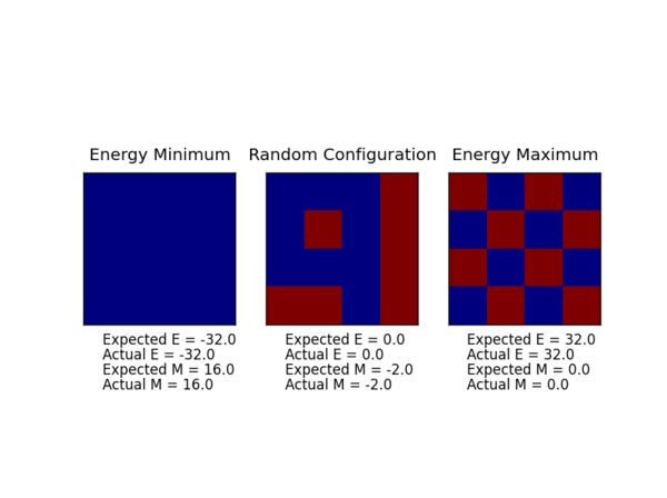
Running the ILcheck.py script tested whether the  energy(self) and magnetisation(self) functions work correctly. The script creates three IsingLattice objects and give the expected results and 
the results from the completed the energy(self) and magnetisation(self) functions. 
As shown above the actual and expected are in agreement, indicating the energy(self) and magnetisation(self) functions work correctly.

Introduction to the Monte Carlo simulation

TASK 6 - How many configurations are available to a system with 100 spins? To evaluate these expressions, we have to calculate the energy and magnetisation for each of these configurations, then perform the sum. Let's be very, very, generous, and say that we can analyse $1 \times 1 0^{9}$ configurations per second with our computer. How long will it take to evaluate a single value of ${⟨ M ⟩}_{T}$ ?

For a system with 100 lattice cells containing spins, we can use a simple statistical thermodynamics equations to obtain the number of possible configurations. The number of states available to each spin is 2, the spin can either be +1 or -1. We have 100 spins in our system, so the total possible configurations/microstates is given by 2¹⁰⁰. It is important to remember that we are not at absolute zero, where the system is constrained to be completely aligned, i.e. where there is only 2 microstates. One method we can use to find the ensemble average for the energy and the net magnetisation is to evaluate the summation directly. If the compute could analyse 10⁹ configurations per second, it would take 1.27 x 10²¹ seconds to evaluate the net magnetization at a given temperature, if we think of this in years, it would take 4.00 x 10¹³ years! Clearly this is computationally impossible and we need another approach to evaluate the E(T) and M(T), we can introduce a clever technique called Importance sampling. For many of the configurations the $\exp {- \frac{E (α)}{k_{B} T}}$ , will be very small, and that state will have negligible contribution to the average value for the property. In importance sampling, we will only sample states that the system is likely to occupy at the given temperature. This approximation is computationally achievable.

TASK 7


def montecarlostep(self, T):
        initial_configuration, energy, magnetisation= self.lattice, self.energy(), self.magnetisation()
        random_i = np.random.choice(range(0, self.n_rows))
        random_j = np.random.choice(range(0, self.n_cols))
        self.lattice[random_i, random_j]=-self.lattice[random_i, random_j]
        random_configuration, random_energy, random_magnetisation= self.lattice, self.energy(), self.magnetisation()
        energy_difference=random_energy-energy
        #the following line will choose a random number in the range [0,1)
        random_number = np.random.random()
        if energy_difference<=0:
            initial_conifguration, energy, magnetisation= random_configuration, random_energy, random_magnetisation
        elif energy_difference>0:
            if np.exp(-energy_difference/T)>=random_number:
                initial_conifguration, energy, magnetisation= random_configuration, random_energy, random_magnetisation
            elif np.exp(-energy_difference/T)<random_number:
                self.lattice[random_i, random_j]=-self.lattice[random_i, random_j]
        self.E, self.E2, self.M, self.M2=self.E+energy, self.E2+energy**2, self.M+magnetisation, self.M2+magnetisation**2
        self.n_cycles+=1
        return energy, magnetisation
        
    def statistics(self):
        aveE = self.E/(self.n_cycles)
        aveE2 = self.E2/(self.n_cycles)
        aveM = self.M/(self.n_cycles)
        aveM2 = self.M2/(self.n_cycles)

        return aveE, aveE2, aveM, aveM2, self.n_cycles

NJ: good!

TASK 8


cycles =  3989
Averaged quantities:
E =  -1.92928992229
E*E =  3.77885767893
M =  -0.964323765355
M*M =  0.946325050138

Output from the statistics function, giving the Average E/per spin and M/per spin from the simulation.

%run ILanim.py runs the simulation and gives the result shown in the PNG image above. It runs the simulation at 0.5 K and after approximately 600 cycles we reach each equilibrium and leave the transient region, with the averages no longer fluctuating (or very negligible changes). The average interaction energy/per spin and the average magnetisation/per spin is reported in the statistics output shown above. Previously we have noted the lowest energy configuration has an energy $- D N J = E$ , for this 8x8 2D Ising lattice we expect an E/per spin of -2 reduced units at 0 K. Our simulation at 0.5 K gives us a value of E = -1.92928992229, which sounds correct and in agreement with our theory from part 1. Similarly the lowest energy configuration will have a magnetisation of either +1 or -1 per spin, and once again at 0.5K the average magnetisation is M = -0.964323765355, which once again is in close agreement to what we should expect at near 0 K temperatures. When the temperature is below the Curie Temperature, T<T_C, we expect spontaneous magnetisation (A net magnetisation). The Averaged M/per spin is non-zero from the statistics function, this suggests we are in an ordered state with net magnetisation, with 0.5 K below the Curie temperature.

NJ: Not Kelvin! Reduced units!

Accelerating the code

TASK 9

The ILtimetrial.py script is used to record how long current version of the IsingLattice.py takes to perform 2000 Monte Carlo algorithm steps. The ILtimetrial.py script was run 10 times with the average taken and the standard error calculated. The following was obtained;

< t i m e t a k e n > = 34.87550295849419 \pm 0.04291393753105752

TASK 10


Below are the "accelerated" energy(self) and magnetisation(sekf) functions!

def energy(self):
        
        horizontal_product= np.sum(np.multiply(self.lattice, np.roll(self.lattice, 1, axis=0)))
        vertical_product= np.sum(np.multiply(self.lattice, np.roll(self.lattice, 1, axis=1)))
        energy=-(horizontal_product +vertical_product)
        return energy


    def magnetisation(self):
        
        magnetisation= np.sum(self.lattice)
        return magnetisation

TASK 11

The ILtimetrial.py script is used to record how long optimised version of the IsingLattice.py takes to perform 2000 Monte Carlo algorithm steps. The ILtimetrial.py script was run 10 times with the average taken and the standard error calculated. The following was obtained;

< t i m e t a k e n > = 0.3992326502097967 \pm 0.0002359318866317137

This average time taken is clearly very much faster than the original energy(self) and magnetisation(self) functions not making use of the NumPy module.

NJ: are you surprised by the difference?

The effect of temperature

TASK 12

Previously, when we ran the ILanim.py and made use of the current statistics() and montecarlostep() functions where the code averages from the beginning. Instead of averaging from the first random configuration, we should only average in the region where the average energy and magnetization are constant, this way our average properties will be more accurate and correct (after an x amount of steps). For this we need to modify our statistics() and montecarlostep() functions so that we only start averaging after the transient period. First we have to determine the number of steps from which the E/M values/per spin are ignored for the averaging purposes.

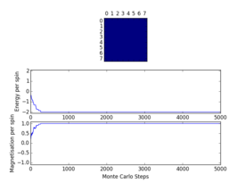
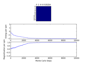
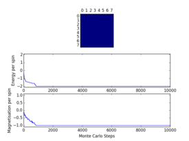
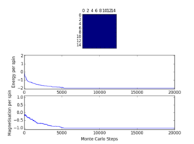
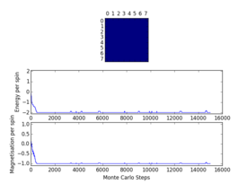
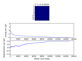
Plots from the ILfinalframe.py script runs at different temperatures/lattice sizes are shown below. This is to determine how many cycles are typically needed for the system to go from its random starting position to the equilibrium state. Below are E/spin and M/spin v number of cycle plots as well as a depiction of the final lattice state.


8x8 lattice at 0.25K	16x16 lattice at 0.25K	8x8 lattice at 0.5K

16x16 lattice at 0.5K	8x8 lattice at 1K	16x16 lattice at 1K

From the plots, we can see that for a 8x8 lattice at all three temperatures tested, the average energy and magnetization always become constant <<2000 cycles. Ignoring the first 2000 cycles would make sure that when we only average in the region where the average energy and magnetization are constant. 16 x 16 Ising lattices were also sampled, and it is clear that it takes considerably more cycles for the for the properties to become constant and no longer be in the transient phase, for example, for the 16 x 16 lattice at 1K, it takes 10000 steps before the properties equilibrate and remain at a constant value. The explanation for this is quite intutitve if you consider the what the algorithm is actually doing. For larger lattices, randomly flip any one of the spin will have a smaller effect on the energy than compared to the before, this makes the condition for the acceptance of the new configuration more likely, hence cause continued fluctuation in the values. From the data above it is sensible to modify the statistics() and montecarlostep() functions so that the first 10000 cycles of the simulation are ignored when calculating the averages (accommodating for varying temperatures and lattice sizes). It was realised later that for the 32x32 ignoring 10,000 cycles was not sufficient, this was confirmed when looking at the heat capacity v temperature plot later in the experiment. It is expected the heat capacity becomes increasingly sharply peaked as the system size was increased, but for the 32x32 this was not the case and it was less sharp than the 16x16. I then changed the period ignored to 30000 and changed the number of cycles in the ILtemperature.py script to 200,000, giving better results!

Below are the corrected statistics() and montecarlostep() functions to take this into account.

 
    E = 0.0
    E2 = 0.0
    M = 0.0
    M2 = 0.0
    equib_period = 0.0

    n_cycles = 0

    def __init__(self, n_rows, n_cols):
        self.n_rows = n_rows
        self.n_cols = n_cols
        self.lattice = np.random.choice([-1,1], size=(n_rows, n_cols))

    def energy(self):
        
        horizontal_product= np.sum(np.multiply(self.lattice, np.roll(self.lattice, 1, axis=0)))
        vertical_product= np.sum(np.multiply(self.lattice, np.roll(self.lattice, 1, axis=1)))
        energy=-(horizontal_product +vertical_product)
        return energy


    def magnetisation(self):
        
        magnetisation= np.sum(self.lattice)
        return magnetisation

    def montecarlostep(self, T):
        initial_configuration, energy, magnetisation= self.lattice, self.energy(), self.magnetisation()
        random_i = np.random.choice(range(0, self.n_rows))
        random_j = np.random.choice(range(0, self.n_cols))
        self.lattice[random_i, random_j]=-self.lattice[random_i, random_j]
        random_configuration, random_energy, random_magnetisation= self.lattice, self.energy(), self.magnetisation()
        energy_difference=random_energy-energy
        #the following line will choose a random number in the range [0,1)
        random_number = np.random.random()
        if energy_difference<=0:
            initial_conifguration, energy, magnetisation= random_configuration, random_energy, random_magnetisation
        elif energy_difference>0:
            if np.exp(-energy_difference/T)>=random_number:
                initial_conifguration, energy, magnetisation= random_configuration, random_energy, random_magnetisation
            elif np.exp(-energy_difference/T)<random_number:
                self.lattice[random_i, random_j]=-self.lattice[random_i, random_j]
        if self.equib_period<10000:
            self.equib_period+=1
        else:
            self.E, self.E2, self.M, self.M2=self.E+energy, self.E2+energy**2, self.M+magnetisation, self.M2+magnetisation**2
            self.n_cycles+=1
        return energy, magnetisation
        
    def statistics(self):
        aveE = 0.0
        aveE2 = 0.0
        aveM = 0.0
        aveM2 = 0.0
        if self.equib_period>=10000:
            aveE = self.E/(self.n_cycles)
            aveE2 = self.E2/(self.n_cycles)
            aveM = self.M/(self.n_cycles)
            aveM2 = self.M2/(self.n_cycles)

        return aveE, aveE2, aveM, aveM2, self.n_cycles

TASK 13 - Use ILtemperaturerange.py to plot the average energy and magnetisation for each temperature, with error bars, for an $8 \times 8$ lattice. Use your initution and results from the script ILfinalframe.py to estimate how many cycles each simulation should be. The temperature range 0.25 to 5.0 is sufficient. Use as many temperature points as you feel necessary to illustrate the trend, but do not use a temperature spacing larger than 0.5. T NumPy function savetxt() stores your array of output data on disk — you will need it later. Save the file as 8x8.dat so that you know which lattice size it came from


Below is the ILtemperaturerange.py script used to plot the average energy/per spin and magnetisation/per spin in the temperature range 0.25 to 5 K. 
A temperature spacing of 0.1 K is used to for give the temperatures at which the script runs the monte carlo simulations.
The script runs 100000 cycles per simulation - enough runs (after the ignored runs) from which accurate averages can be calculated to give E/per spin and M/per spin.
Below the script is the PNG file for the resulting plot for the 8x8 lattice size.


from IsingLattice import *
from matplotlib import pylab as pl
import numpy as np

n_rows = 8 #manually change these
n_cols = 8
il = IsingLattice(n_rows, n_cols)
il.lattice = np.ones((n_rows, n_cols))
spins = n_rows*n_cols
runtime = 100000
times = range(runtime)
temps = np.arange(0.25, 5.0, 0.1)
energies = []
magnetisations = []
energysq = []
magnetisationsq = []
ener_error, mag_error = [], []

for t in temps:
    for i in times:
        if i % 100 == 0:
            print(t, i)
        energy, magnetisation = il.montecarlostep(t)
    aveE, aveE2, aveM, aveM2, n_cycles = il.statistics()
    energies.append(aveE)
    energysq.append(aveE2)
    ener_error.append(((aveE2-(aveE**2))**0.5)/(spins*(n_cycles**0.5)))
    magnetisations.append(aveM)
    magnetisationsq.append(aveM2)
    mag_error.append(((aveM2-aveM**2)**0.5)/(spins*(n_cycles**0.5)))
    #reset the IL object for the next cycle
    il.E = 0.0
    il.E2 = 0.0
    il.M = 0.0
    il.M2 = 0.0
    il.n_cycles = 0
fig = pl.figure()
enerax = fig.add_subplot(2,1,1)
enerax.set_ylabel("Energy per spin")
enerax.set_xlabel("Temperature")
enerax.set_ylim([-2.1, 2.1])
magax = fig.add_subplot(2,1,2)
magax.set_ylabel("Magnetisation per spin")
magax.set_xlabel("Temperature")
magax.set_ylim([-1.1, 1.1])
enerax.plot(temps, np.array(energies)/spins)
magax.plot(temps, np.array(magnetisations)/spins)
enerax.errorbar(temps, np.array(energies)/spins, yerr=np.array(ener_error), color="b", marker="o")
magax.errorbar(temps, np.array(magnetisations)/spins, yerr=np.array(mag_error), color="r", marker="o")
pl.show()

final_data = np.column_stack((temps, energies, energysq, magnetisations, magnetisationsq))
np.savetxt("8x8.dat", final_data)


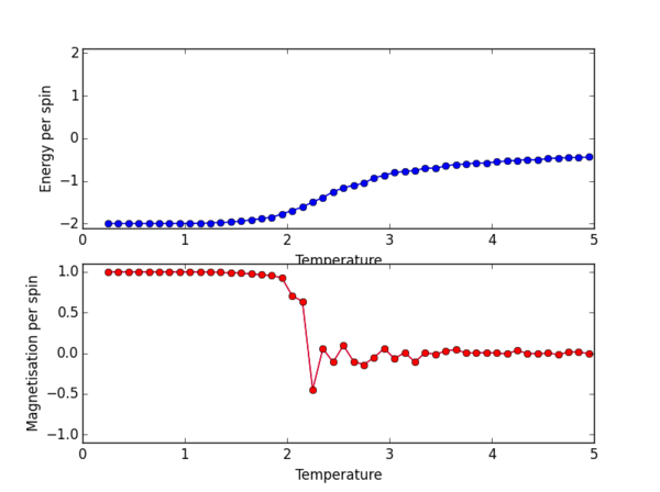
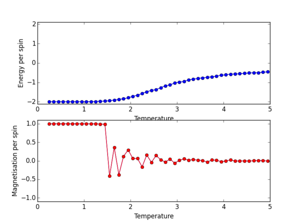
The plot for the 8 x 8 lattice shows a clear transition at the Curie temperature.
By eye we can estimate this to be around 2.3ish, but we can definitely confirm that the phase
transition from ordered spins to disorded spins occurs between 2-3 K. Once the 
Magnetisation per spin is 0 we can confirm that we have indeed passed the Curie 
temperature, as the Ising lattice no longer has a net magnetisation.

The effect of system size

TASK 14 - Repeat the final task of the previous section for the following lattice sizes: 2x2, 4x4, 8x8, 16x16, 32x32. Make sure that you name each datafile that your produce after the corresponding lattice size! Write a Python script to make a plot showing the energy per spin versus temperature for each of your lattice sizes. Hint: the NumPy loadtxt function is the reverse of the savetxt function, and can be used to read your previously saved files into the script. Repeat this for the magnetisation. As before, use the plot controls to save your a PNG image of your plot and attach this to the report. How big a lattice do you think is big enough to capture the long range fluctuations?

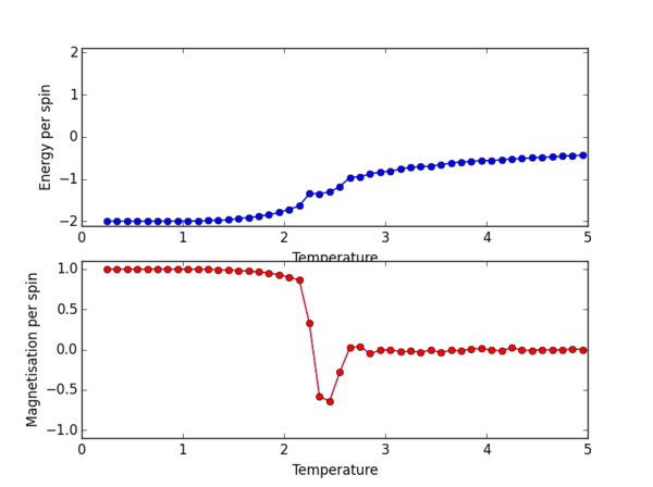
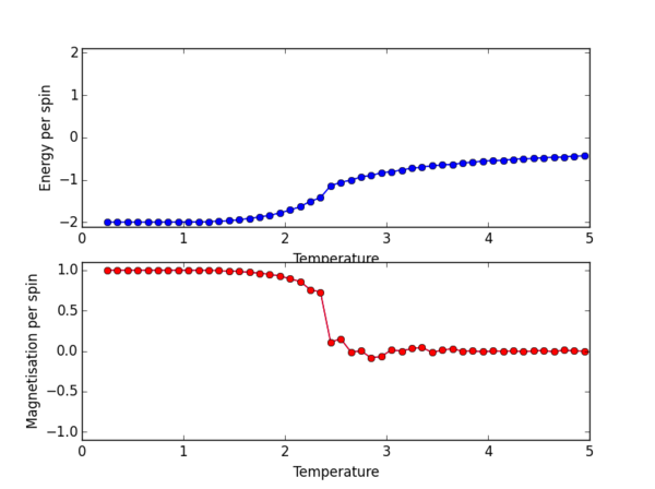
The ILtemperaturerange.py script was again used, now to plot for the 2x2, 4x4, 16x16, 32x32 lattice sizes. PNG files for the E/spin and M/spin v temperature
graphs are given below for these lattice sizes, the plots for the 8x8 lattice is also given again for comparison.
From the M/spin v Temperature plots we can see the onset of a phase transition from the ferromagnetic ordered phase to a disordered phase
where the system results in no net magnetisation. The regions on the M/spin v Temperatures plots where the magnetisation fluctuates extensively and eventually
equilibrates around 0 is the temperature range across which the phase transition is occuring. In this region, the energetic and entropic driving forces are of almost equal
importance. At the lower temperatures, we have the system which is almost uniformly aligned across the entire lattice. This is confirmed because we have M/spin at low
temperatures around 1. At these low temperatures the energetic driving force prevails since there is not enough energy in the system to overcome the favourable interactions
between the adjacent aligned spins. At the higher temperatures, the entropic driving force prevails, the system has enough energy to begin flipping slips which begins to considerably
increase the entropy of the two energy level system. The system becomes disordered with high entropy, randomly aligned spins, and hence a M/per spin of around 0.

The plots for the different lattice sizes vary in two ways, as we increase the lattice size the phase transition begins at a higher temperature. Secondly, the temperature ranges
for fluctuations corresponding to the phase transitions also vary. The 16x16 plots and the 32x32 plot show no significant change in the temperature range across which fluctuations
begin to take place, indicating that the 16x16 lattice size is sufficient in modelling the long range fluctuations.

NJ: Nice plots — a plot of E vs T for all lattice sizes on the same axes would make the trend easier to see; the 8x8 lattice actually gives similar results to the 16x16.

2 x 2

4 x 4

8 x 8

16 x 16

32 x 32

Determining the Heat Capacity

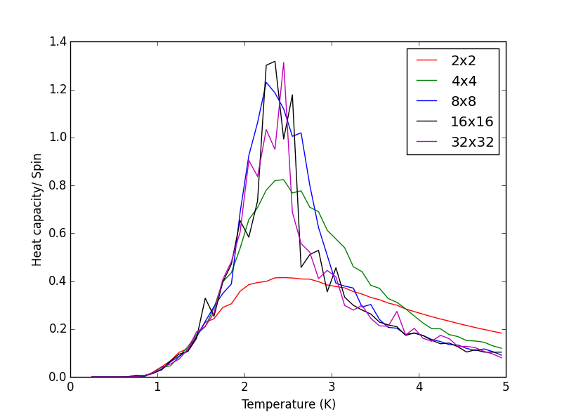
TASK 15 - Write a Python script to make a plot showing the heat capacity versus temperature for each of your lattice sizes from the previous section. You may need to do some research to recall the connection between the variance of a variable, $V a r [X]$ , the mean of its square $⟨ X^{2} ⟩$ , and its squared mean ${⟨ X ⟩}^{2}$ . You may find that the data around the peak is very noisy — this is normal, and is a result of being in the critical region. As before, use the plot controls to save your a PNG image of your plot and attach this to the report.

The script heatcapacity.py, shown below was used to obtain the Heat capacity/spin v Temperature plots for 
the different sizes of the Ising lattice. The scripts uses the data files saved by the ILtemperaturerange.py
code in the previous task. The PNG file below the heatcapacity.py script, shows a single plot for the 2x2, 4x4, 
8x8, 16x16 and 32x32 lattice sizes.

from IsingLattice import *
from matplotlib import pylab as pl
import numpy as np

rows = [2, 4, 8, 16, 32]
colours = ['r', 'g', 'b', 'k', 'm']
n=0

fig=pl.figure()
for row in rows:
    values = np.loadtxt(str(row)+"x"+str(row)+".dat")
    temperatures = values[ : ,0]
    heat_capacity = np.subtract(values[ : , 2], (values[ : , 1])**2)/(temperatures**2)
    hc = fig.add_subplot(1,1,1)
    hc.set_ylabel("Heat capacity/ Spin")
    hc.set_xlabel("Temperature (K)")
    c=colours[n]
    hc.plot(temperatures, heat_capacity/(row**2), c, label=str(row)+"x"+str(row))
    n+=1

pl.legend()
pl.show()

Locating the Curie temperature

TASK 16

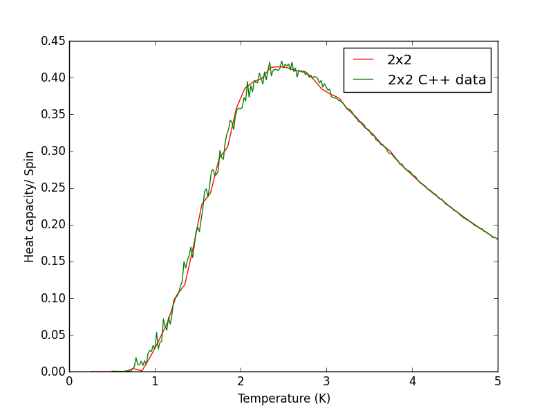
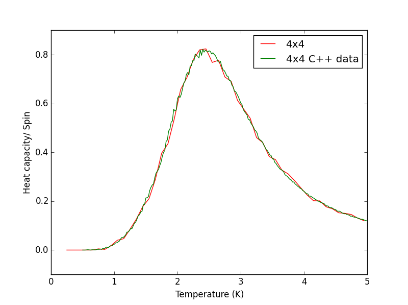
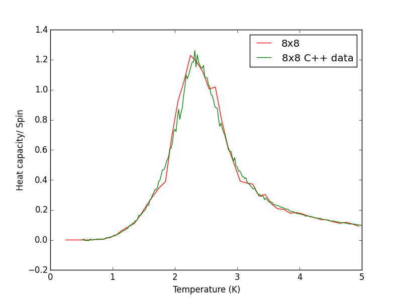
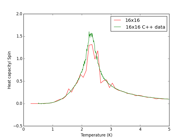
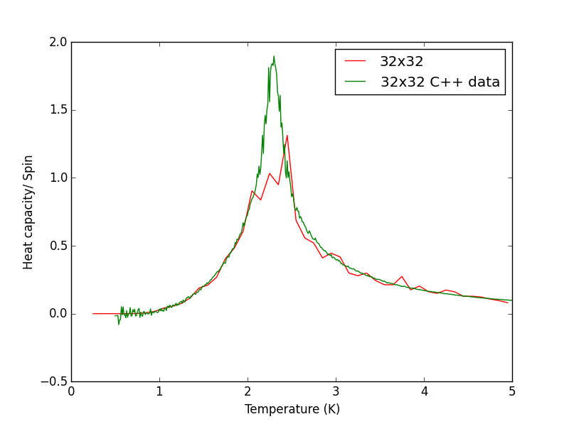
Script to plot C++ data against own data for different lattice sizes, the lattice size for which the 
script plots is changed manually. PNG files showing plots for the 2x2, 4x4, 8x8, 16x16 and 32x32 lattices
are given below this script.


from IsingLattice import *
from matplotlib import pylab as pl
import numpy as np

rows = [2]
colours = ['r', 'g']
n=0

fig=pl.figure()
for row in rows:
    values = np.loadtxt(str(row)+"x"+str(row)+".dat")
    values_from_C = np.loadtxt("../ImperialChem-Year3CMPExpt-master/C++_data/"+str(row)+"x"+str(row)+".dat")
    temperatures = values[ : ,0]
    temperatures_C = values_from_C[ : ,0]
    heat_capacity = np.subtract(values[ : , 2], (values[ : , 1])**2)/(temperatures**2)
    heat_capacity_C = values_from_C[ : , 5]
    hc = fig.add_subplot(1,1,1)
    hc.set_ylabel("Heat capacity/ Spin")
    hc.set_xlabel("Temperature (K)")
    hc.plot(temperatures, heat_capacity/(row**2), colours[n], label=str(row)+"x"+str(row))
    hc.plot(temperatures_C, heat_capacity_C, colours[n+1], label=str(row)+"x"+str(row)+" C++ data")
    
    

pl.legend()
pl.show()

TASK 17 - write a script to read the data from a particular file, and plot C vs T, as well as a fitted polynomial. Try changing the degree of the polynomial to improve the fit — in general, it might be difficult to get a good fit! Attach a PNG of an example fit to your report


The following script is used read the C++ data, plot C vs T data, as well as a fitted polynomial. The degree of
polynomial and the C++ data used (depending on lattice size) are manually controlled. 
The code was run to find the best fitting polynomial for each lattice size, PNG files are attached below.

from IsingLattice import *
from matplotlib import pylab as pl
import numpy as np

rows=8 #manually change this
data_C=np.loadtxt("../ImperialChem-Year3CMPExpt-master/C++_data/"+str(rows)+"x"+str(rows)+".dat")
T=data_C[:, 0]
C=data_C[:, 5]    
fig = pl.figure()
heat_capacity_plot = fig.add_subplot(1,1,1)
heat_capacity_plot.set_ylabel("Heat Capacity/ Spin")
heat_capacity_plot.set_xlabel("Temperature")

poly_degree=3 #manually change this 
fit = np.polyfit(T, C, poly_degree)

T_min = np.min(T)
T_max = np.max(T)
T_range = np.linspace(T_min, T_max, 1000) 
fitted_C_values = np.polyval(fit, T_range)
heat_capacity_plot.plot(T_range, fitted_C_values, label=str(rows)+"x"+str(rows)+"polynomial degree: "+str(poly_degree))
heat_capacity_plot.plot(T, C, color="r", label=str(rows)+"x"+str(rows)) 
heat_capacity_plot.legend(loc=2, prop={'size':7})

pl.show()


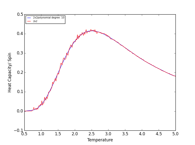
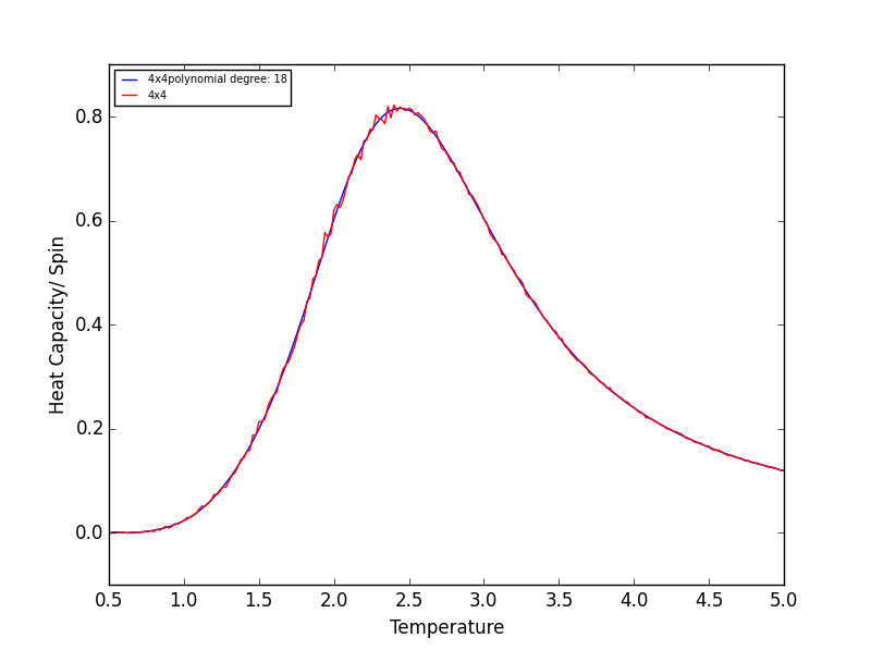
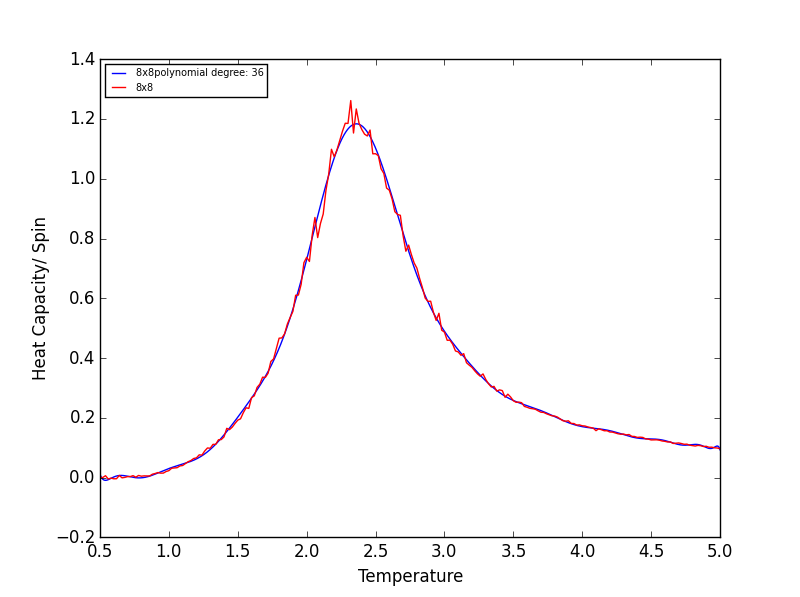
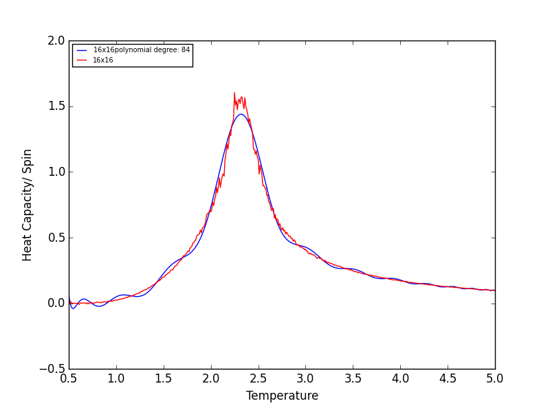
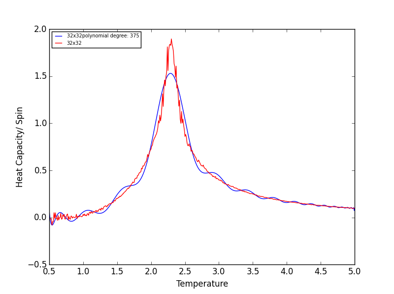
Quick note on the above graphs - for all the lattice sizes there were large ranges of polynomial degrees which gave effectively the same fit. If all the polynomials across these
range of degrees were plotted on a single graph they would overlap! The degree of the polynomials shown in the above graphs give as good fit as any other!

TASK 18 - Modify your script from the previous section. You should still plot the whole temperature range, but fit the polynomial only to the peak of the heat capacity! You should find it easier to get a good fit when restricted to this region.


Rather than having a fitted polynomial across the entire temperature range of the C++ data, 
fitting to a particular range may allow us to find a better fitting polynomials for the Heat Capacity v Temperature data.
The script below is a modified version of the script used in the previous section which allows fitting of the 
polynomial in a chosen temperature range - the region in which the Heat capacity peaks!


from IsingLattice import *
from matplotlib import pylab as pl
import numpy as np

rows=32 #manually change this
data_C=np.loadtxt("../ImperialChem-Year3CMPExpt-master/C++_data/"+str(rows)+"x"+str(rows)+".dat")
T=data_C[:, 0]
C=data_C[:, 5]    
fig = pl.figure()
heat_capacity_plot = fig.add_subplot(1,1,1)
heat_capacity_plot.set_ylabel("Heat Capacity/ Spin")
heat_capacity_plot.set_xlabel("Temperature")

T_min = 2.15 #manually change these if required to get a better polynomial fit 
T_max = 2.45

selection = np.logical_and(T > T_min, T < T_max) #choose only those rows where both conditions are true
peak_T_values = T[selection]
peak_C_values = C[selection]

poly_degree=18 #manually change this 
fit = np.polyfit(peak_T_values, peak_C_values, poly_degree)

T_min = np.min(peak_T_values)
T_max = np.max(peak_T_values)
T_range = np.linspace(T_min, T_max, 1000) 
fitted_C_values = np.polyval(fit, T_range)
heat_capacity_plot.plot(T_range, fitted_C_values, label=str(rows)+"x"+str(rows)+"polynomial degree: "+str(poly_degree)+ " T: "+str(T_min)+"-"+str(T_max))
heat_capacity_plot.plot(T, C, color="r", label=str(rows)+"x"+str(rows)) 
heat_capacity_plot.legend(loc=2, prop={'size':7})

pl.show()


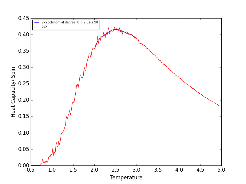
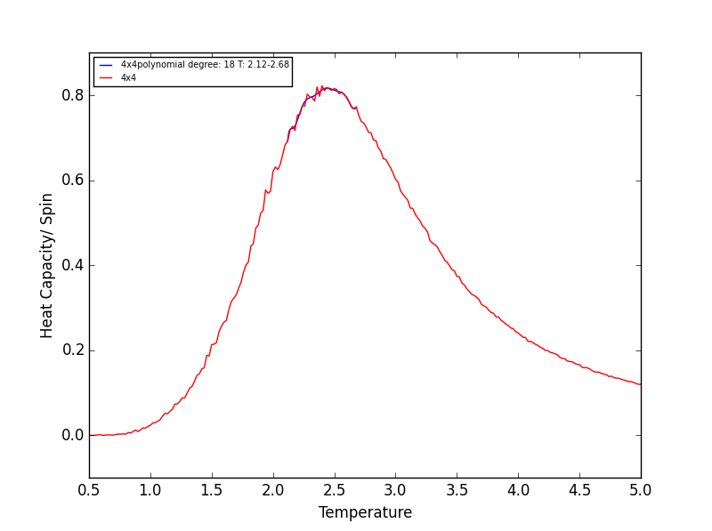
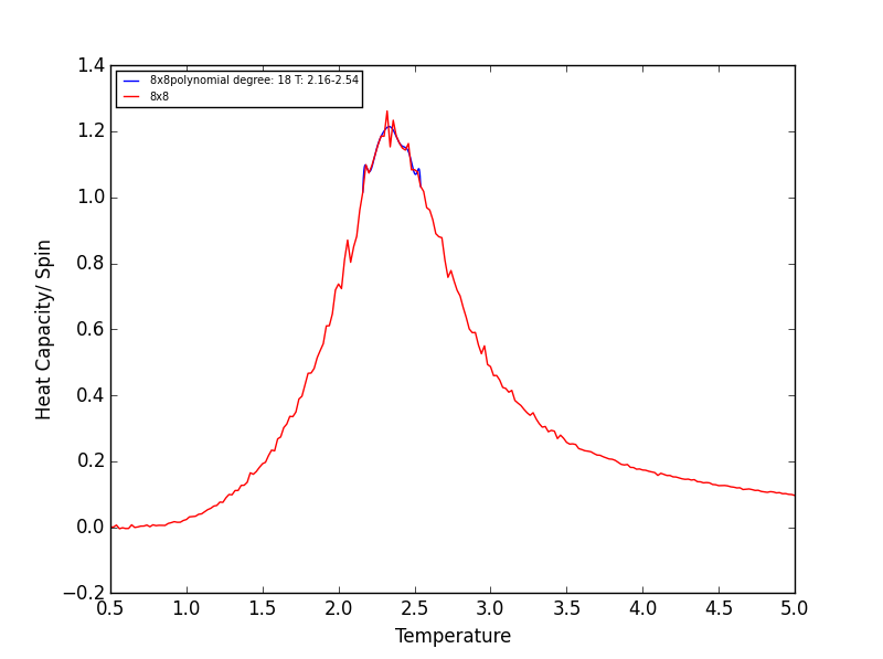
Quick note on the above plots - Once again the temperature ranges chosen and the degree of the polynomial combined gave a fit as good as any other combination! Plotting a series of polynomials 
with varying degrees (that fit well) would simply overlap!
For the next task these fitted polynomials are adequate.

TASK 19 - find the temperature at which the maximum in C occurs for each datafile that you were given. Make a text file containing two colums: the lattice side length (2,4,8, etc.), and the temperature at which C is a maximum. This is your estimate of $T_{C}$ for that side length. Make a plot that uses the scaling relation given above to determine $T_{C, \infty}$ . By doing a little research online, you should be able to find the theoretical exact Curie temperature for the infinite 2D Ising lattice. How does your value compare to this? Are you surprised by how good/bad the agreement is? Attach a PNG of this final graph to your report, and discuss briefly what you think the major sources of error are in your estimate.


The script below finds the maximum in C from our fitted polynomials for each lattice size, and the corresponding temperature.
This temperature is our experimental Curie Temperature for the varying lattice sizes. The final part of the script saves a text file
containing two columns: the lattice side length (2,4,8, etc.), and the Experimental Curie temperature, which is required in the final task.


from IsingLattice import *
from matplotlib import pylab as pl
import numpy as np

l_rows=[2, 4, 8, 16, 32]
degrees=[8,18,18,18,18] #the degrees here correspond to the polynomial degrees in the previous task  
l_T_min=[2.02,2.12,2.16,2.16,2.16] #to correspond with the range fitted to from the previous task 
l_T_max=[2.98,2.68,2.54,2.54,2.44] #to correspond with the range fitted to from the previous task 
n=0
T_c=[]

for rows in l_rows:
    data_C=np.loadtxt("../ImperialChem-Year3CMPExpt-master/C++_data/"+str(rows)+"x"+str(rows)+".dat")
    T=data_C[:, 0]
    C=data_C[:, 5]    
    
    T_min = l_T_min[n] 
    T_max = l_T_max[n]

    selection = np.logical_and(T > T_min, T < T_max) #choose only those rows where both conditions are true
    peak_T_values = T[selection]
    peak_C_values = C[selection]

    fit = np.polyfit(peak_T_values, peak_C_values, degrees[n])

    T_min = np.min(peak_T_values)
    T_max = np.max(peak_T_values)
    T_range = np.linspace(T_min, T_max, 1000) 
    fitted_C_values = np.polyval(fit, T_range)

    Cmax = np.max(fitted_C_values)
    Tmax = T_range[fitted_C_values == Cmax]
    T_c.append(Tmax)
    n+=1


final_data = np.column_stack((l_rows, T_c))
np.savetxt("T_c_data_task19.dat", final_data)


This final script below uses the text files from the previous task and plots the scaling relation given below, 
from this the experimental Curie temperature for an infinite 2D Ising lattice can be calculated.

$T_{C, L} = \frac{A}{L} + T_{C, \infty}$


from IsingLattice import *
from matplotlib import pylab as pl
from numpy import *
import numpy as np

fig = pl.figure()
data=np.loadtxt("T_c_data_task19.dat")
temps=data[ : , 1]
rows=data[ : , 0]

fit = np.polyfit(1/rows, temps, 1)

x_values=np.linspace(0, np.max(1/rows), 1000)
line_params = np.polyval(fit, x_values)
plot_box = dict(boxstyle='round', facecolor='yellow', alpha=0.5)
plot_box_text=("Curie Temperature: {}".format(fit[1]))


ax = fig.add_subplot(1,1,1)
ax.set_ylabel("Curie temperature (K)")
ax.set_xlabel("1/L")
ax.text(0.05, 0.95, plot_box_text, transform=ax.transAxes, fontsize=11, verticalalignment='top', bbox=plot_box)
ax.plot(1/rows, temps, "g", linestyle="", marker="o")
ax.plot(x_values, line_params, "r")

pl.show()

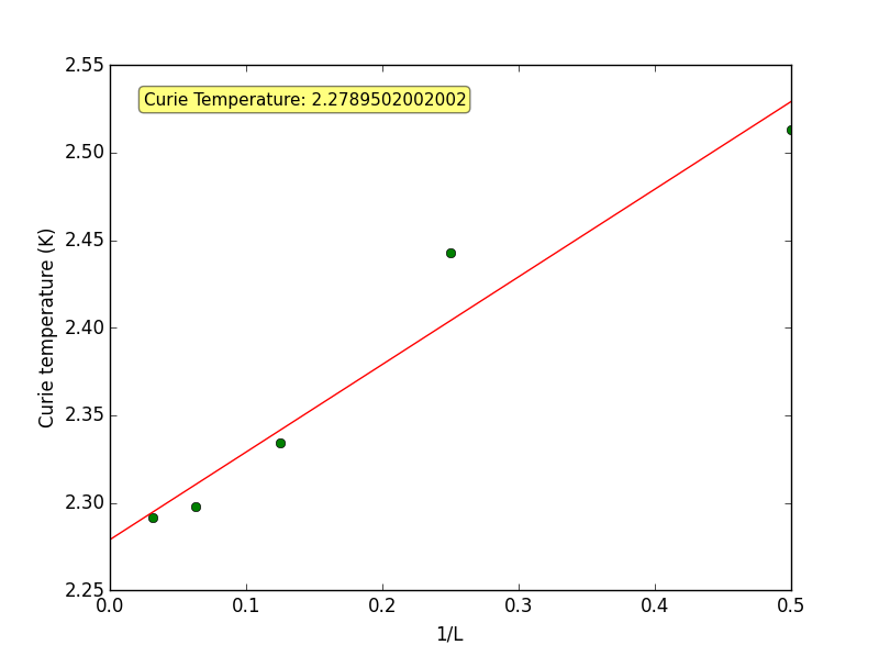
It is known that the two way infinite Ising lattice has a order/disorder transition at a temperature $T = T_{C}$ given by the condition $s i n h (\frac{2 J}{k_{B} T_{c, \infty}}) s i n h (\frac{2 J^{'}}{k_{B} T_{c, \infty}}) = 1$ . ^[1] For this experiment, we set $K_{B} = 1$ and $J = J^{'} = 1$ .

The above equation can now be written $s i n h^{2} (\frac{2}{T_{c, \infty}}) = 1$

Solving;

$T_{c, \infty} = 2.26919 K$ (Theoretical)

$T_{c, \infty} = 2.27900 K$ (Experimental)

Commentary and Sources of error

The experimental and theoretical values are in close agreement and the same to 1 decimal place, however there is still a noticeable discrepancy between the
two due to various sources of error. Assuming that the C++ data was also derived from a Monte Carlo simulation; The amount of cycles ignored and the number
of cycles used to eventually obtain the Heat Capacity v Temperature data would have been important. If some values which are part of the transient region are
incorporated when averaging, the energy/per spin values across the temperature range would have some degree of inaccuracy. This data was then processed
and presented in the form it was given to us in. A similar reasoning can be applied to the length of the simulation used to obtain the C++ data. We have been
told that these were much longer simulations than possible on college computers and so extensive error deriving from this argument is unlikely!

The main source of error would come from the polynomial we used to model the C++ data for the different lattice sizes. We fitted polynomials to a specific temperature
range, rather than the whole range to obtain much tighter and better fits. Shrinking the temperature domain to which the polynomials fit would perhaps given much better
fitted polynomials - giving a better indication of the maxima in heat capacity and hence the Curie temperatures for the different lattice sizes.
Perhaps using a function which outputs the best R<sup>2</sup> of the polynomial through simulation across varying Tmin-Tmax values and polynomial degrees could
gives the very very best fit for the data! But this will be limited as it still depends on how good the raw C++ data is in the first place.

NJ: one problem is that this function isn't really a polynomial, so we can only make an approximate fit.

Instead of having 5 lattice sizes, perhaps 10 or 15 different sizes would be useful, since this would add more points to graph we used to determine the Curie temperature
for the infinite lattice (intercept), the more points we could observe a better straight line fit for the <math>T_{C, L} = \frac{A}{L} + T_{C,\infty}</math> function.

NJ: Good. You could also ignore the results from the very small lattices.


The sources of error are a combination of the how computationally strict the C++ simulations where in addition to how good the fitted polynomials were, which 
in turn were used to find the Curie temperatures for the 2x2, 4x4, 16x16 and 32x32 lattice sizes.

References

↑ L. Onsager, Phys. Rev, 1944, 65, 117

[1] L. Onsager, Phys. Rev, 1944, 65, 117

[1]