Simulation of a Simple Liquid

Numerical Intergration

TASK: Open the file HO.xls. In it, the velocity-Verlet algorithm is used to model the behaviour of a classical harmonic oscillator. Complete the three columns "ANALYTICAL", "ERROR", and "ENERGY": "ANALYTICAL" should contain the value of the classical solution for the position at time $t$ , "ERROR" should contain the absolute difference between "ANALYTICAL" and the velocity-Verlet solution (i.e. ERROR should always be positive -- make sure you leave the half step rows blank!), and "ENERGY" should contain the total energy of the oscillator for the velocity-Verlet solution. Remember that the position of a classical harmonic oscillator is given by $x (t) = A \cos (ω t + ϕ)$ (the values of $A$ , $ω$ , and $ϕ$ are worked out for you in the sheet).

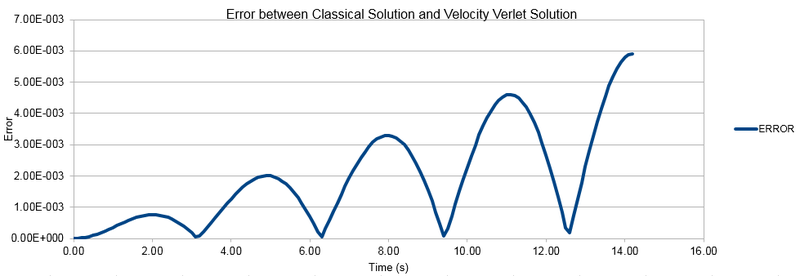
The graphs below show the results of each column, Analytical, Error and Energy versus time.

TASK: For the default timestep value, 0.1, estimate the positions of the maxima in the ERROR column as a function of time. Make a plot showing these values as a function of time, and fit an appropriate function to the data.

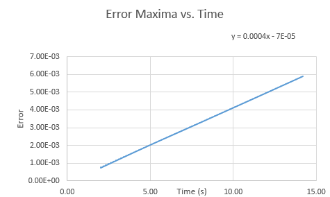
The graph below shows the the maxima of the error versus time with the function written on the graph.

NJ: Why do you think the error keeps accumulating like this?

TASK: Experiment with different values of the timestep. What sort of a timestep do you need to use to ensure that the total energy does not change by more than 1% over the course of your "simulation"? Why do you think it is important to monitor the total energy of a physical system when modelling its behaviour numerically?

After experimenting with different timesteps it was found that a timestep of 0.0968 gave a maximum error of 0.005 which is 1% of the total energy 0.5. Therefore, any timestep under this value will give an error of less than 1%. The Error vs Time is shown below:

NJ: This question is about the error in the energy, not the position.

It is important to monitor the total energy of a system as we expect energy to be conserved. If this is not the case and energy is increasing or decreasing it can be a sign that our system is not stable and has not reached equilibrium. Fluctuation around an average energy is to be expected as the particles move and interact but overall it should remain constant.

NJ: Good

Atomic Forces

The quantum physics needed to work out the forces acting upon a set of atoms can't be solved easily so approximations are made. From classical physics the force acting on an object is given as:

F_{i} = - \frac{d U (r^{N})}{d r_{i}}

$r^{N}$ stands for the position vectors of every atom in system. The force that a single atom feels is determined by the position of every other atom. Finding a function $U$ that includes all the key physics of the interatomic interactions in the system for simple liquids can be achieved using the Lennard-Jones potential. $U$ therefore can be written as:

U (r^{N}) = \sum_{i}^{N} \sum_{i \neq j}^{N} {4 ϵ (\frac{σ^{12}}{r_{i j}^{12}} - \frac{σ^{6}}{r_{i j}^{6}})}

'TASK: For a single Lennard-Jones interaction, $ϕ (r) = 4 ϵ (\frac{σ^{12}}{r^{12}} - \frac{σ^{6}}{r^{6}})$ , find the separation, $r_{0}$ , at which the potential energy is zero. What is the force at this separation? Find the equilibrium separation, $r_{e q}$ , and work out the well depth ( $ϕ (r_{e q})$ ). Evaluate the integrals $\int_{2 σ}^{\infty} ϕ (r) d r$ , $\int_{2.5 σ}^{\infty} ϕ (r) d r$ , and $\int_{3 σ}^{\infty} ϕ (r) d r$ when $σ = ϵ = 1.0$ .

a) When potential energy is zero:

$0 = 4 ϵ (\frac{σ^{12}}{r^{12}} - \frac{σ^{6}}{r^{6}})$

$0 = \frac{σ^{12}}{r^{12}} - \frac{σ^{6}}{r^{6}}$

$\frac{σ^{12}}{σ^{6}} = \frac{r^{12}}{r^{6}}$

$σ^{6} = r^{6}$

$σ = r$

The force at this separation can then be worked out using the above differential:

$F_{i} = - 4 ϵ (\frac{- 12 σ^{12}}{r_{0}^{13}} - \frac{6 σ^{6}}{r_{0}^{7}})$

Substituting $σ$ for r gives us:

$F_{i} = - 4 ϵ (\frac{- 12}{σ} + \frac{6}{σ})$

$F_{i} = \frac{24 ϵ}{σ}$

b) The equilibrium separation is the minimum of the curve. We can take the first derivative of our equation and equal the force to zero, the value of r is therefore the equilibrium separation.

$0 = 4 ϵ (\frac{- 12 σ^{12}}{r_{0}^{13}} - \frac{6 σ^{6}}{r_{0}^{7}})$

$2 σ^{6} = r^{6}$

$2^{1 / 6} σ = r$

c) Substituting the equilibrium value of r into the Lennard-Jones formula gives us the well depth:

$ϕ = 4 ϵ (\frac{σ^{12}}{(2^{1 / 6} σ)^{12}} - \frac{σ^{6}}{(2^{1 / 6} σ)^{6}})$

This gives:

$ϕ = - ϵ$

Below the integrals in the task are evaluated with $σ = ϵ = 1.0$

$\int_{2 σ}^{\infty} ϕ (r) d r = - 0.025$

$\int_{2.5 σ}^{\infty} ϕ (r) d r = - 8.17 x 1 0^{- 3}$

$\int_{3 σ}^{\infty} ϕ (r) d r = - 3.29 x 1 0^{- 3}$

NJ: Good - I would like to have seen the working for the integrals, though.

Periodicity Boundary Conditions

TASK:Estimate the number of water molecules in 1ml of water under standard conditions. Estimate the volume of 10000 water molecules under standard conditions.

a) First we must work out the number of moles of water in 1ml. Water has a molecular mass of 18g/mol. As 1ml of water weighs one gram, if we divide 1 by 18 we get the number of moles which equals 0.056. Multiplying this by Avogadro's number gives the number of water molecules:

0.056 x 6.022×10²³ = 3.35x10²² molecules.

b) As 1ml of water equals 1g, if we work out the weight of 10000 water molecules we get the volume. The number of moles in 10000 molecules equals:

10000/6.022×10²³ = 1.66x10^-20moles

Multiplying this by the molecular mass of water equals:

1.66x10^-20 x 18g/mol = 2.99x10^-19g

The volume of water therefore equals 1.66x10^-20cm³

NJ: No, 2.99e-19 mL - 1g per mL.

TASK: Consider an atom at position \left(0.5, 0.5, 0.5\right) in a cubic simulation box which runs from \left(0, 0, 0\right) to \left(1, 1, 1\right). In a single timestep, it moves along the vector \left(0.7, 0.6, 0.2\right). At what point does it end up, after the periodic boundary conditions have been applied?

As the box runs from (0, 0, 0) to (1, 1, 1) when the atom is moved along each coordinate it stays in the same box. For example, moving 0.7 along the x axis from 0.5 would give us 1.2, but as this is not allowed in the confines of the box the resulting x value is 0.2. Therefore for all axis, the resulting point is (0.2, 0.1, 0.7). NJ: Good

Reduced Units

TASK:The Lennard-Jones parameters for argon are $σ = 0.34 n m, ϵ = 120 / k_{B} K$ . If the LJ cutoff is $3.2 σ$ , what is it in real units? What is the well depth in ${k J m o l}^{- 1}$ ? What is the reduced temperature $T^{*} = 1.5$ in real units?

a) Multiplying the sigma value for argon and the LJ cut-off gives the real units of:

3.2 x 0.34nm = 1.088nm

b) We know from previous tasks that $ϕ = - ϵ$ . Therefore the well depth is -120/k_BK. To convert this to kJ mol^-1 we must multiply by k_B and N_A and then divide by 1000 to give the correct units:

-120 x k_B x N_A/1000 = -0.10 Kj mol^-1

NJ: It's about 1, so you've lost a factor of ten somewhere here.

c) The reduced temperature can be written as:

T^{*} = T k_{b} / ϵ

Therefore multiplying T^* by epsilon gives us the temperature:

1.5 x 120 = 180K

Equilibration

Creating the simulation box

TASK:Why do you think giving atoms random starting coordinates causes problems in simulations? Hint: what happens if two atoms happen to be generated close together?

If two atoms are generated close together their potentials can overlap leading to a high energy state not found a real liquid and ultimately repulsion. It is therefore better to place the atoms in a cubic lattice and allow them to reach equilibrium so they arrange themselves into more realistic configurations.

NJ: Good. Why do you think this problem wouldn't just go away by itself as the simulation runs - the atoms will repel each other if they are too close, after all.

TASK: Satisfy yourself that this lattice spacing corresponds to a number density of lattice points of 0.8. Consider instead a face-centred cubic lattice with a lattice point number density of 1.2. What is the side length of the cubic unit cell?

The input file has the line:

'lattice sc 0.8'

This defines the lattice to be a cubic lattice with a number density of 0.8. The lattice spacing is also defined, with one line of our log output file reading:

 'Lattice Spacing in x,y,x = 1.07722 1.07722 1.07722'

We can confirm that this separation does indeed correspond to a number density of 0.8. The side lengths of the unit cell would be equal to 1.07722. The volume of a cubic cell is A³ therefore the volume of this cell would equal 1.07722³ which equals 1.25. There is only one atom in a cubic lattice unit cell so as:

Number density = Number of atoms/Volume

If we divide 1 by 1.25 we then get the density of 0.8.

A face centered cubic unit cell has 4 atoms in each unit: each of the 8 corners gives 0.25 and each of the 4 centered atoms give 0.5 to the cell. (8 x 0.25)+(4 x 0.5) = 4. Using the above equation, dividing the number of atoms by the number density of 1.2 gives the volume of 3.33. Taking the cube root of this value will give us the cell length: 3.33⅓ = 1.49.

TASK: Consider again the face-centered cubic lattice from the previous task. How many atoms would be created by the create_atoms command if you had defined that lattice instead?

In our input file there is the command:

region box block 0 10 0 10 0 10
create_box 1 box

Our log file has the corresponding line:

Created orthogonal box = (0 0 0) to (10.7722 10.7722 10.7722)

This command gives us a box of 10x10x10 unit cells, and as each cell contains one atom, 1000 atoms. If we were to instead use a face-centered cubic lattice as mentioned before, our 10x10x10 lattice would contain 4000 atoms.

NJ: Good.

Setting the properties of the atoms

TASK: Using the LAMMPS manual, find the purpose of the following commands in the input script:

mass 1 1.0
pair_style lj/cut 3.0
pair_coeff * * 1.0 1.0

a) mass I value is the generic format for the script above, setting the mass for all atoms. I can be a numeric value or a 'wild-card asterisk' such as 'n' or '*' can be used to set the mass for multiple atom types. The value is a the mass of the atom.

b) pair_style style args is the generic format of this script. This denotes the interaction between a pair of atoms. Here, lj/cut 3.0 refers to a Lennard Jones interactions between the two atoms with a cut off of 3.0 distance units.

c) pair_coeff I J args is the generic format of this script with I and J being atom types and args being the force field coefficients of I and J. Above the '* *' is used to set the coefficients for all I,J pairs, and the '1.0 1.0' setting them both to 1.0.

NJ: What are the coefficients that are being set?

TASK: Given that we are specifying $x_{i} (0)$ and $v_{i} (0)$ , which integration algorithm are we going to use?

We will use the Velocity Verlet Algorithm as this includes both the position x(0) and the velocity v(0) while the Verlet algorithm only specifies the position x(0).

Running the Simulation

TASK: Look at the lines below.

### SPECIFY TIMESTEP ###
variable timestep equal 0.001
variable n_steps equal floor(100/${timestep})
variable n_steps equal floor(100/0.001)
timestep ${timestep}
timestep 0.001

### RUN SIMULATION ###
run ${n_steps}
run 100000

The second line (starting "variable timestep...") tells LAMMPS that if it encounters the text ${timestep} on a subsequent line, it should replace it by the value given. In this case, the value ${timestep} is always replaced by 0.001. In light of this, what do you think the purpose of these lines is? Why not just write:

timestep 0.001
run 100000

The timestep is repeated many times throughout the script when referenced to other commands. This value needs to be kept constant throughout therefore writing out the full definition of the timestep ensures this so that there is no need to keep defining it in further coding.

NJ: This section makes sure that the simulation always simulates the same length of time, no matter what timestep is chosen.

Checking equilibration

TASK: make plots of the energy, temperature, and pressure, against time for the 0.001 timestep experiment (attach a picture to your report). Does the simulation reach equilibrium? How long does this take? When you have done this, make a single plot which shows the energy versus time for all of the timesteps (again, attach a picture to your report). Choosing a timestep is a balancing act: the shorter the timestep, the more accurately the results of your simulation will reflect the physical reality; short timesteps, however, mean that the same number of simulation steps cover a shorter amount of actual time, and this is very unhelpful if the process you want to study requires observation over a long time. Of the five timesteps that you used, which is the largest to give acceptable results? Which one of the five is a particularly bad choice? Why?

Below are the plots of energy, temperature and pressure against time for the 0.001 timestep experiment.

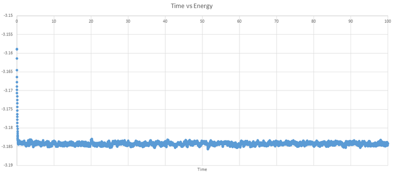
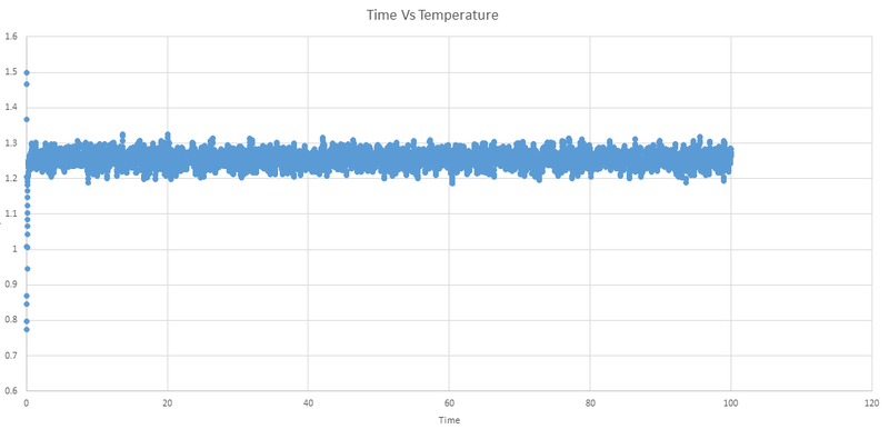
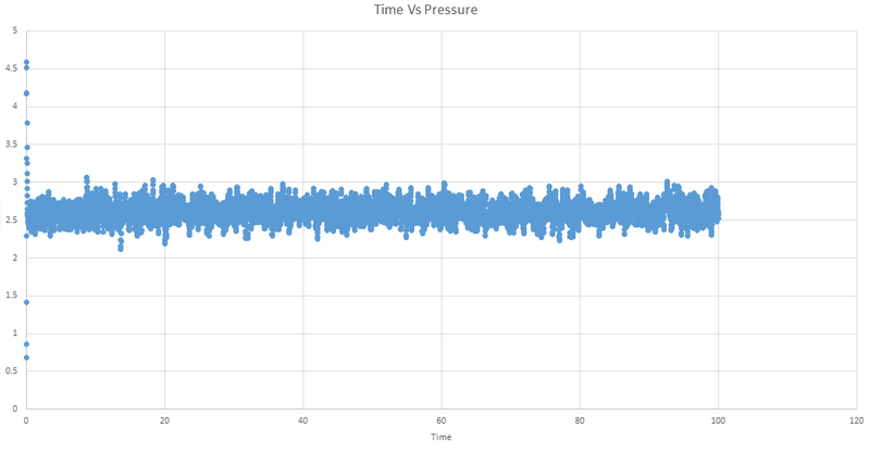
We can see that the system does reach equilibrium, and by zooming in on the first graph we can estimate this time to be around 0.4 seconds.

The graph below shows the Time vs Energy plots for the timesteps 0.001, 0.0025, 0.0075, 0.01 and 0.015.

The timesteps in the range of 0.001-0.01 all reach equilibrium and show similar results with and energy ranges less than 0.05 units apart. The simulation of the 0.015 timestep does not reach equilibrium and instead becomes unstable and increases rapidly. This makes it an unsuitable choice for a simulation.

NJ: Good, 0.015 is the really poor choice. The question also asks which is the largest choice that gives acceptable results.

Simulations Under Specific Conditions

Temperature and Pressure Control

TASK: Choose 5 temperatures (above the critical temperature $T^{*} = 1.5$ ), and two pressures (you can get a good idea of what a reasonable pressure is in Lennard-Jones units by looking at the average pressure of your simulations from the last section). This gives ten phase points — five temperatures at each pressure. Create 10 copies of npt.in, and modify each to run a simulation at one of your chosen $(p, T)$ points. You should be able to use the results of the previous section to choose a timestep. Submit these ten jobs to the HPC portal. While you wait for them to finish, you should read the next section.

For these ten simulations I have chosen the timestep of 0.0025 after looking at the results of the previous section. The temperatures; 1.6, 1.8, 2.0, 2.2 and 2.4 were chosen with the pressures of 2.5 and 2.8 after looking at the pressures of the output files from previous simulations.

Thermostats and Barostats

TASK: We need to choose $γ$ so that the temperature is correct $T = 𝔗$ if we multiply every velocity $γ$ . We can write two equations:

$\frac{1}{2} \sum_{i} m_{i} v_{i}^{2} = \frac{3}{2} N k_{B} T$

$\frac{1}{2} \sum_{i} m_{i} {(γ v_{i})}^{2} = \frac{3}{2} N k_{B} 𝔗$

Solve these to determine $γ$ .

To determine $γ$ we can divide equation 2 by equation one resulting in:

γ^{2} = T / 𝔗

Taking the square root therefore gives us:

γ =

(T/

𝔗

)^½

NJ: Good, but I would like to see a little more working.

Examining the Input Script

TASK: Use the manual page to find out the importance of the three numbers 100 1000 100000. How often will values of the temperature, etc., be sampled for the average? How many measurements contribute to the average? Looking to the following line, how much time will you simulate?

a) 100 refers to Nevery: a command that uses input values every specified timesteps, in this instance 100. 1000 refers to Nrepeat: the number of times to use the input values for calculating averages. 100000 refers to Nfreq: this command calculates averages every 100000 timesteps in this script.

b) The temperature will therefore be sampled every 100 timesteps for the average.

c) 1000 measurements will therefore be used for the average.

d) As the run lasts 100000 timesteps and one average is calculated every 100000 timesteps, only one average will be calculated. As the timestep chosen was 0.0025, the amount of time simulated will be 0.0025 x 100000 = 250 seconds.

NJ: Be careful, the time is 250 "time units", not 250 seconds. All of the units in this exercise are reduced.

Plotting the Equations of State

TASK: When your simulations have finished, download the log files as before. At the end of the log file, LAMMPS will output the values and errors for the pressure, temperature, and density $(\frac{N}{V})$ . Use software of your choice to plot the density as a function of temperature for both of the pressures that you simulated. Your graph(s) should include error bars in both the x and y directions. You should also include a line corresponding to the density predicted by the ideal gas law at that pressure. Is your simulated density lower or higher? Justify this. Does the discrepancy increase or decrease with pressure?

a)Below shows the graphs for T vs N/V at pressures of 2.5 and 2.8.

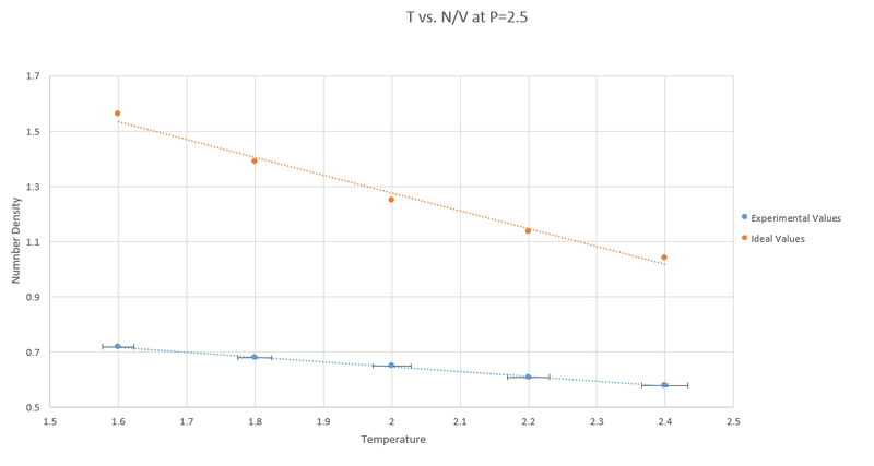
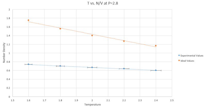
The table below shows the error for each graph in the experimental values:

Temperature	1.6	1.8	2.0	2.2	2.4
T Error at P = 2.5	0.0226	0.0247	0.0279	0.0305	0.0338
N/V Error at P= 2.5	0.0041	0.0041	0.0041	0.0045	0.0041
T Error at P = 2.8	0.0229	0.0253	0.0291	0.0314	0.0330
N/V Error at P = 2.8	0.0040	0.0041	0.0041	0.0041	0.0050

b) The Experimental values are all lower than the values calculated by the ideal gas law (N/V = P/T). This is because the ideal gas law does not take into account interactions between atoms and once this is factored in the number density decreases as repulsive interactions mean atoms are less likely to be found close together. NJ: Good

c)The discrepancies decrease with pressure as at higher pressures the atoms are forced closer together therefore behaving more like an ideal gas. NJ: Your data shows that the discrepancy increases with pressure. Does what you've said make sense? Are denser gasses usually more or less ideal? What happens as the temperature changes?

Calculating Heat Capacities using Statistical Physics

TASK: As in the last section, you need to run simulations at ten phase points. In this section, we will be in density-temperature $(ρ^{*}, T^{*})$ phase space, rather than pressure-temperature phase space. The two densities required at $0.2$ and $0.8$ , and the temperature range is $2.0, 2.2, 2.4, 2.6, 2.8$ . Plot $C_{V} / V$ as a function of temperature, where $V$ is the volume of the simulation cell, for both of your densities (on the same graph). Is the trend the one you would expect? Attach an example of one of your input scripts to your report.

An example script for the density 0.8 at temperature 2.8 can be found here

The graph below shows the collated data from the ten inputs, 5 at the pressure 0.2 and 5 at 0.8:

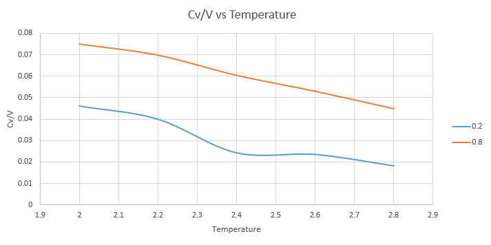
NJ: You shouldn't just join up the points with smooth lines in situations like this - do you think the "bump" is really part of the trend, or due to experimental error?

We can see from the graph that the heat capacity is larger when the density is higher. This is to be expected; at a higher density there are more atoms per volume and as heat capacity is directly related to the number of molecules it will be higher.

NJ: Yes, heat capacity is extensive. What about the variation with temperature?

Structural Properties and the Radial Distribution Function

TASK: perform simulations of the Lennard-Jones system in the three phases. When each is complete, download the trajectory and calculate $g (r)$ and $\int g (r) d r$ . Plot the RDFs for the three systems on the same axes, and attach a copy to your report. Discuss qualitatively the differences between the three RDFs, and what this tells you about the structure of the system in each phase. In the solid case, illustrate which lattice sites the first three peaks correspond to. What is the lattice spacing? What is the coordination number for each of the first three peaks?

a)The radial distribution functions for a solid, gas and liquid were collated below. The solid had a fcc lattice with a density of 1.2 and a temperature of 1.0. The gas had a density of 0.2 and a temperature of 2.5, and the liquid had a density of 0.2 and a temperature of 1.0.

NJ: Strictly speaking, you have a fluid, not a gas, under the conditions you gave (supercritical). This is unlikely to affect your results. A density of 0.2 wouldn't give a liquid, but I think this is a typo

b)From the graphs we can see that they all have a neighbour close to them initially. For the gas function, this then tails off with no further peaks. We can infer that there is one initial neighbour and then a long time before another is found - correct with what we know about the disperse nature of gases. Looking at the liquid function, there is a second peak and almost a third. It has more closer neighbours than a gas but if we compare to the solids radial distribution function it is still only near a few molecules at a time. The solids function supports what we know about lattices with periodic peaks suggesting a highly structured system.

NJ: You've got the right general idea, but be careful with your terminology - the RDF x axis is distance, not time. So for the gas you could say that there is a first nearest neighbour at a distance of about 1, but that there is no structure beyond that. The first liquid peak actually look to be a little further away the gas peak, so you can't really say that the first neighbour is closer. Why do you think the RDF begins with a value of 0? NJ: We would generally describe the RDFs as follows: the gas is structurally disordered (one well defined nearest neighbour, beyond which the disposition of atoms is essentially random); the liquid has short range order (between 2 and 3 coordination shells), but no long range order; finally, the solid has both short and long range order.

c) The picture below depicts which lattice sites the first three points correspond to.

d) We can work out the coordination number for each peak and the lattice spacing by investigating the first three minimum of the RDF for the solid. These integrals can be found by corresponding the the reduced unit at the minimum and using the graph below to find the integration of the area below.

The first three minimum correspond to distances of 1.275, 1.675 and 1.975. When extrapolated from the graph above this gives 12.01, 17.97 and 42.26. By subtracting the previous integrals from these values (ie subtract 12.01 from 17.97) we get the rounded coordination numbers of 12, 6 and 24. We know that the second peak must correspond to the atom in the corner of the cube, as it is the closest to our initial atom. The distance of this atom is therefore the length of the cube, and so the lattice spacing is 1.675.

NJ: Do you mean maxima instead of minima? You found that the lattice spacing was 1.675, but earlier you worked out that it should be about 1.5 for an FCC lattice of this density. Why do you think this might be? You can work out what the distance to each of the three neighbours should be in terms of a, the lattice spacing, and then average the three values.

Dynamical Properties and the Diffusion Coefficient

Mean Squared Displacement

TASK: make a plot for each of your simulations (solid, liquid, and gas), showing the mean squared displacement (the "total" MSD) as a function of timestep. Are these as you would expect? Estimate $D$ in each case. Be careful with the units! Repeat this procedure for the MSD data that you were given from the one million atom simulations.

a) Below are the graphs for the Mean Squares Distribution for solid liquid and gas:

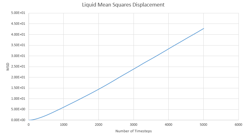
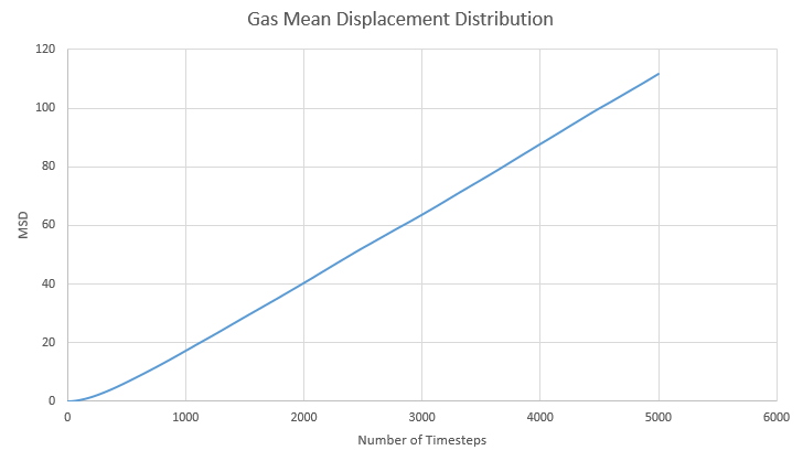
b) In the solid lattice movement is restricted as each atom is tightly packed together. This is then shown as a very small diffusion coefficient and agrees with theory. Atoms in a liquid have more freedom to move but the interactions between atoms mean that they never completely separate. This is reflected in the diffusion coefficient being much larger than in the solid. In a gas complete separation is found as gas atoms can freely move far apart from each other. We can see the effect of this with the largest diffusion coefficient out of the three.

NJ: What do you mean by separate? This one is more about density. The less dense your system is, the further an atom can travel before it collides with another one. That generally means that its average speed will be larger.

c) D can be estimated by the gradient of each graph once it has reached equilibrium. Using the equation below we can divide the slope by six:

D = \frac{1}{6} \frac{\partial ⟨ r^{2} (t) ⟩}{\partial t}

This table shows the gradient and final D value for each graph.

State	Gradient	D
Solid	1.05x10^-8	1.31x10^-9
Liquid	9.41x10^-3	1.57x10^-3
Gas	2.40x10^-2	4.01x10^-3

NJ: These values are all "per-timestep". You need to convert the x axis to time units to get the true diffusion constant.

d)The MSD graphs for the one million atom simulations are shown below:

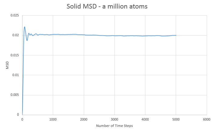
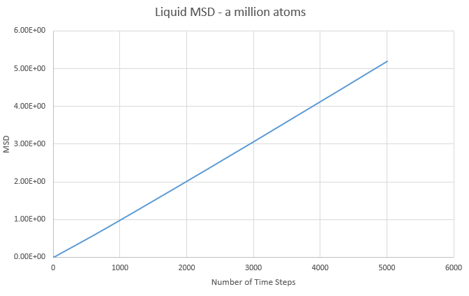
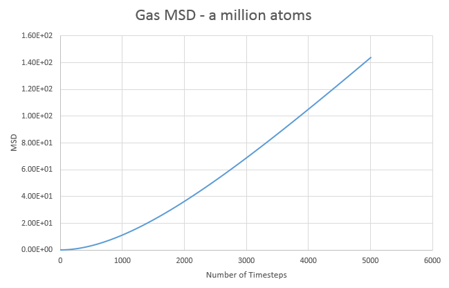
State	Gradient	D
Solid	1.08x10^-7	1.81x10^-8
Liquid	1.06x10^-3	1.78x10^-4
Gas	3.65x10^-2	6.09x10^-3

Overall the graphs show similar trends, with the million atom graphs showing smoother lines, as to be expected with more data and averages available. Comparing both sets of data we see that the liquid diffusion constant gets smaller with more atoms in the simulation while both the gas and solid diffusion constants get larger with more atoms in the simulation.

NJ: What do you mean by "smoother lines"? They all look quite smooth. In this case, the gas MSD is quite curved - what do you think is happening there? Remember that you don't know what conditions the million atom simulations were performed at - that might explain the differences.

Velocity Autocorrelation Function

Part 1

TASK: In the theoretical section at the beginning, the equation for the evolution of the position of a 1D harmonic oscillator as a function of time was given. Using this, evaluate the normalised velocity autocorrelation function for a 1D harmonic oscillator (it is analytic!):

$C (τ) = \frac{\int_{- \infty}^{\infty} v (t) v (t + τ) d t}{\int_{- \infty}^{\infty} v^{2} (t) d t}$

Be sure to show your working in your writeup. On the same graph, with x range 0 to 500, plot $C (τ)$ with $ω = 1 / 2 π$ and the VACFs from your liquid and solid simulations. What do the minima in the VACFs for the liquid and solid system represent? Discuss the origin of the differences between the liquid and solid VACFs. The harmonic oscillator VACF is very different to the Lennard Jones solid and liquid. Why is this? Attach a copy of your plot to your writeup.

a) From our previous task we know that $x (t) = A \cos (ω t + ϕ)$ and that the velocity of this harmonic oscillator is = v = dx/dt. If we differentiate the equation above we get:

v(t) = -Aωsin(ωt + φ)

Therefore:

v(t + г) = -Aωsin(ω(t + г) + phi)

We can combine these equations with the original integral to give: NJ: Be careful with the minus signs. This looks like you have two terms in the integrand, one subtracted from the other.

This can be rearranged to give: NJ: No negative in front

Knowing that sin(a+b)= sin(a)cos(b)+ cos(a)sin(b):

This can be rearranged to:

This can be simplified into two fractions:

The first fraction cancels to cos(ωt). The second fraction cannot be cancelled. If we inspect the numerator we see the function is odd, when integrated will give an answer of zero. It does not matter the value of the denominator as we know we can't have infinity as an answer (i.e 0/x) so we can cancel out the whole second fraction to give:

C(г) = cos(ωt)

NJ: Good. This is well explained apart from the two minor notation issues. b) Using the above formula with ω =½π, the simple harmonic oscillator was plotted onto the graph below with the VACFs of the solid and liquid.

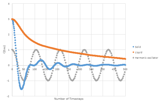
NJ: You could use a line here, rather than points, because you know the functions are continuous. Both plots show some negative minimas as they oscillate around zero. These minimas correspond to negative correlation to the initial velocity due to collisions which produce backward scatters of particles with deflections of nearly 180°. The harmonic oscillator ignores interactions with other particles and so remains periodic and constant throughout. NJ: It's not constant, but yes, that's the reason the correlations never decay to zero.This is not the same for the liquid and solid plot which change throughout. At first they both show a sharp drop as particle interactions and collisions change the velocity. The solid plot has a slower drop, this is understandable as a solid has few collisions with other atoms than a liquid which has more freedom to move.

NJ: Is that true? Which has more nearest neighbours? The solid plot shows the lattice constraints as it resembles a damped version harmonic oscillator more closely than the liquid plot.

Part 2

TASK: Use the trapezium rule to approximate the integral under the velocity autocorrelation function for the solid, liquid, and gas, and use these values to estimate $D$ in each case. You should make a plot of the running integral in each case. Are they as you expect? Repeat this procedure for the VACF data that you were given from the one million atom simulations. What do you think is the largest source of error in your estimates of D from the VACF?

Below show the VACF plots of the solid, liquid and gas data with their corresponding plots of the running integral calculated by the trapezium rule. For the solid data:

For the liquid data:

For the gas data:

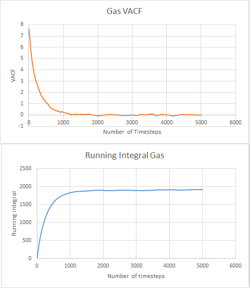
The values for where the running integrals equilibrated were calculated and divided by three to give the diffusion coefficients. This gave values of -0.025, 256.634 and 635.819 for solid, liquid and gas respectively. This follows what we expect with the largest diffusion coefficient being for gas and then liquid with solid having the lowest with the most restrictions of movement.

This was repeated with the data for 1 million atoms. The graphs are shown below. For the solid data:

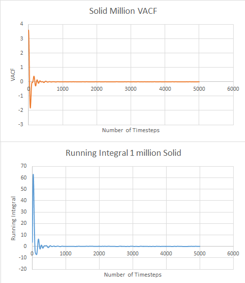
For the liquid data:

For the vapour data:

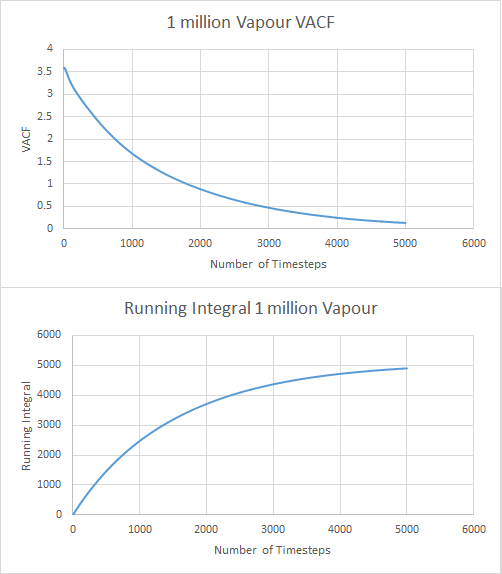
The values for the diffusion coefficient were calculated as before and found to be 0.006, 44.877 and 1563.701 for solid, liquid and vapour respectively. There is a large difference between results for calculating D with the MSD, with many orders of magnitude difference. The trapezium rule is only an estimation of area and so gives us many errors in results. NJ: It's unlikely to cause errors of this magnitude though. This could also be explained by the length of time the VACF takes to reach zero which can lead to a large overestimation of the integral and therefore a larger diffusion coefficient. NJ: Excellent observation - that is the main source of error in the VACF estimate (but it's not why they don't agree). I'd like to see more explanation of this though. MSD only relies on the gradient of the graph which is irrelevant to time, making the VACF estimation much larger than the MSD. NJ: Not really - if you run a longer simulation, there will be less error in the gradient of the MSD.

Overall:

State	D from MSD	D from VACF
Solid	1.31x10^-9	-0.025
Solid 1 million	1.81x10^-8	0.006
Liquid	1.57x10^-3	256.634
Liquid 1 million	1.78x10^-4	44.877
Gas	4.01x10^-3	635.819
Gas 1 million	6.09x10^-3	1563.701

NJ: The results don't agree because both diffusion coefficient are out by a factor of the timestep - the MSD results are one timestep too small, whereas the VACF results are a timestep too big. You ened to convert the x axes to time, not number of timesteps, for the results to make sense.