Talk:Mod:sfs114
JC: General comments: All tasks attempted, but a few mistakes and some answers could have done with a bit more detail. Make sure you understand the theory behind the tasks and ask yourself whether your results are what you would expect.
Theory
Numerical Integration
The classical solution for the position at time compares well with the velocity-Verlet solution:

The total energy for the oscillator varies as shown:

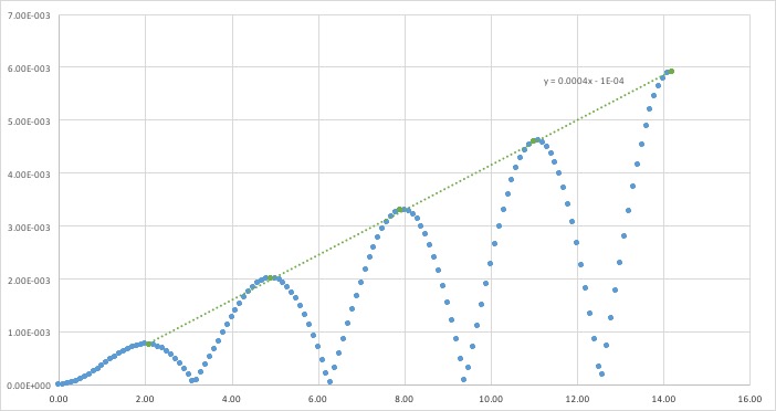
An approximate linear fit has been performed on the maxima of the error of the calculations; the absolute difference between classical and velocity-Verlet solutions. Iterations of using previous results causes error to propagate and increase.
JC: Why does the error oscillate?
The smaller the timestep, the smaller fluctuations in total energy. Calculations over larger timesteps causes a greater error, as particles could end up too close together and face extremely large forces, for example. It is important to monitor the total energy of a physical system to ensure energy is conserved, however infinitesimal timesteps greatly increase time needed to run simulations. Larger timesteps allow a longer length of time to be simulated. A timestep of 0.028s allows energy fluctuations to be as low as of the average value.


Atomic Forces
For a single Lennard-Jones interaction, .
- When potential energy is 0, φ(r) = 0 and r=r0
- If ,
- The force is given by and at a potential energy of 0, .
- At equilibrium separation , .
- At equilibrium separation, the well depth:
- and given that so
JC: All maths correct and clear.
Periodic Boundary Conditions
As , the number of water molecules in 1 mL of water is approximately and 10000 molecules takes up an approximate volume of .
JC: Show more working here, your values are not exactly right.
In a simulation box which runs from (0,0,0) to (1,1,1), an atom that starts at (0.5,0.5,0.5) and moves along vector (0.7,0.6,0.2), will end up at (0.2,0.1,0.7) once periodic boundary conditions have been applied.
Reduced Units
The LJ parameters for Argon are: .
- .
- .
- .
JC: Correct.
Equilibriation
Creating the Simulation Box
If two atoms are generated too close together, the LJ potential shows that the potential between the two would be infinitely large, making force simulations between these two atoms too large to realistically simulate. The LJ cutoff also ensures that LJ potentials are only calculated for atoms that are near enough, and not every other atom in the infinitely repeating lattice, which would greatly increase simulation run time.
JC: Large repulsive forces cause the simulation to crash.
A lattice spacing of 1.07722 corresponds to a lattice number density of for a simple cubic lattice. A face centred cubic lattice has 4 lattice points per cell, and thus would require a lattice spacing of . A 10x10x10 box would contain 1000 unit cells, and 4000 lattice points, so the create_atoms command for such a lattice would create 4000 atoms.
Setting the Properties of the Atoms
The command mass 1 1.0 assigns all atoms of type 1 a mass of 1.0. The command pair_style lj/cut 3.0 defines the cutoff distance between atoms that have a potential between them to be 3.0 (ie. the simulation does not run for atoms farther apart or closer than this distance). The command pair_coeff ** 1.0 1.0 specifically defines the pairwise force field coefficients for multiple pairs atoms.
JC: What do you mean "the simulation does not run for atoms farther apart or closer than this distance"? The force field parameters for a Lennard Jones simulation are epsilon and sigma.
The velocity-Verlet algorithm is the numerical integration method that will be used if and are defined.
Running the Simulation
Calling upon variables, instead of assigning numbers, makes it much easier to change these variables for every simulation that is run.
JC: Why?
Checking Equilibriation
The simulation takes about 0.3 seconds to equilibriate energy, temperature, and pressure, as shown below:
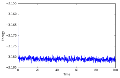
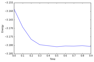

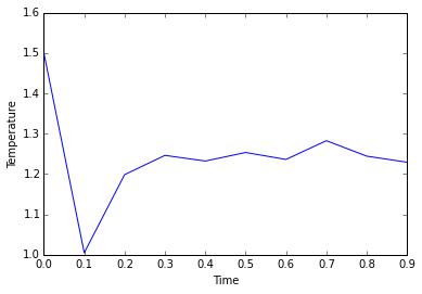
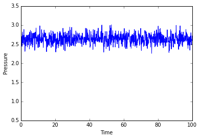
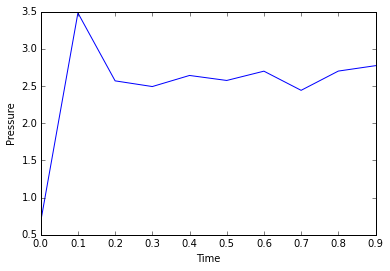

Of the five timsteps used, 0.0025 is the largest acceptable timestep to use as a smaller timestep of 0.001 results in a very similar equilibriation, so going this small is not necessary. 0.015 does not equilbriate at all as the time steps are too large for the numerical integration to accurately find an average for the ensemble, and energy drifts; diverging instead of converging to an average value.
JC: Good choice of timestep, but why not 0.0075 or 0.01? Should the average total energy depend on the choice of timestep?
Running Simulations Under Specific Conditions
Thermostats & Barostats
Examining the Input Script
The command fix aves all ave/time 100 1000 100000 means that values will be sampled every 100 timesteps; in total 1000 readings will be taken to compute a final average on the 100000th timestep.
run 100000 indicates that 100000 timesteps will be simulated.
Plotting the Equations of State
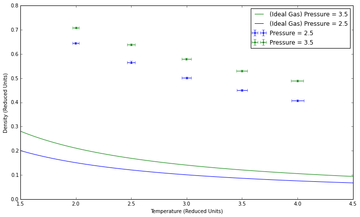
Higher pressures lead to higher densities, both in theory and in these simulations. Our simulated density is higher than that given by the ideal gas law because the simulation takes particle interactions into account. The error increases at higher pressures, when more collisions are likely to occur, while lower pressures would theoretically behave more as an ideal gas would. For the same reason, error decreases at higher temperatures.
JC: Why does the lack of interactions in the ideal gas mean that it has a lower density than the simulations? The lack of repulsion between particles in an ideal gas should mean that this has a higher density than the simulations. What value of kB did you use, remember it should be in reduced units to match the simulation data.
Calculating Heat Capacities Using Statistical Physics

Higher pressure results in higher heat capacity as the increased number of molecules per unit volume that can absorb energy to their vibrational excited states. As the simulation is in a lattice, rotational degrees of freedom are not available to the atoms, and so heat capacity decreases as temperature increases, despite expectations. Alternatively, increasing temperature causes a decrease in band gap, requiring less energy to enter excited states and thus lowering heat capacity.
JC: Good ideas, more analysis beyond this experiment would be needed to properly understand this trend.
An example of the input scripts is below:
Structural Properties and the Radial Distribution Function

The RDF shows the probability of finding a particle at a distance r from a reference particle, relative to an ideal gas. In a gas, there is little order and minimal structure to particles and so the graph has minimal features.
Liquids are slightly more ordered and the decreasing heights of peaks of the RDF correlate to coordination spheres. There is a high probability of finding another particle in a primary coordination sphere but this probability decreases as you go farther away from the reference particle, indicated by decreasing heights of peaks.
The solid FCC lattice has a much higher order, and the RDF peak separation and heights define the lattice structure. The first, second, and third sharp peaks refer to different sets of nearest neighbours, while their heights show how many of those nearest neighbours there are. The lattice spacing is the same as the distance to the second nearest neighbour, 1.475. This agrees well with the original input density of 1.3 (which should result in a lattice spacing of 1.45).
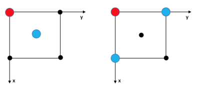

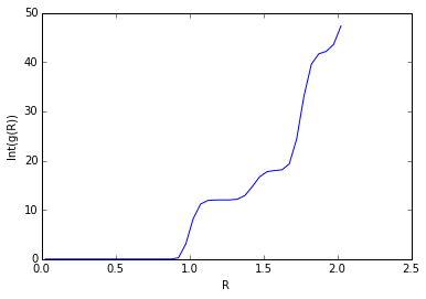
The coordination numbers are 12 (Int(g(1.205)=12, 12 neighbours), 6 (Int(g(1.475)=18, 18-12=6 neighbours), and 24 (Int(g(1.775)=42, 42-18=24 neighbours) respectively.
JC: Good explanation of your results and nice use of fcc diagram. Could you have calculated the lattice spacing from the first and third peak as well and then taken an average?
Dynamical Properties and the Diffusion Coefficient
Mean Squared Displacement
The diffusion coefficient increases as entropy of the phase increases, which matches expectations as gas particles are much more likely to diffuse than a rigid lattice of solid molecules.
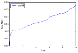


1000000 Atoms

The MSD graph for a gas is curved at first, indicating ballistic motion proportional to . After enough collisions have occurred, diffusion is linear, as it is for a liquid which constantly has the same collisions. The diffusion coefficient is close to 0 for solids which is as expected.
JC: Show the lines of best fit that you've used to calculate D on the graphs. Why does the MSD for your solid data increase over time, is this for an fcc lattice?
Velocity Autocorrelation Function
- and
- sin(x) is an odd function and integrating between and will result in 0
JC: You can simplify the derivation and avoid the intergration if you can identify terms in the integral as odd or even functions and then simplify them accordingly.
VACF minima refer to collisions of particles where velocity is instantaneously 0, negative as they are in the opposite direction. As VACF is averaged over all molecules, they cancel out once they are out of phase, which happens faster for liquids than it does for solids. In comparison to the harmonic oscillator, which only models one particle without any collisions, no convergence to 0 occurs.
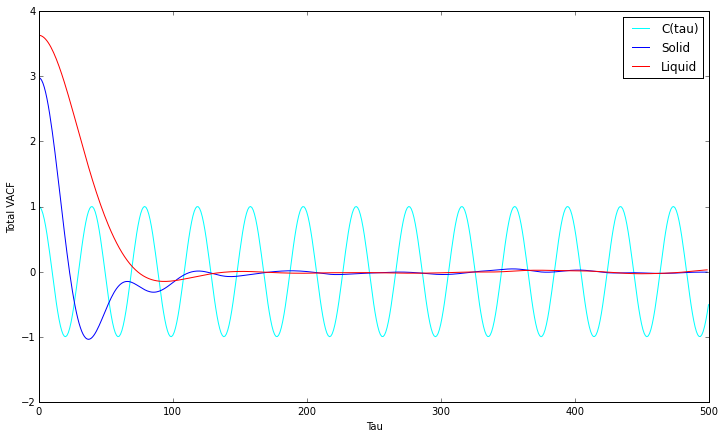
Diffusion coefficient estimations, using the trapezium rule:


1000000 Atoms

- The trapezium rule estimation of the integral for a solid was found to be -0.416 for 1000000 atoms between 0 and 500. (D would hypothetically equal -0.139)

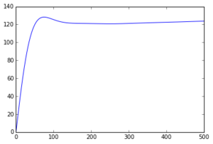

The estimated diffusion coefficients for the two simulations follow the same trend, however the values obtained for the larger 1000000 atom simulations are generally smaller. The largest sources of error include the trapezium rules used to calculate the integral and the simulation assumption that velocities do not change upon collisions.
JC: Check captions in these figures.
