Talk:Mod:scotthuang

JC: General comments: All tasks completed, but it would be good to include a sentence or two after some tasks to show that you understand the significance of your data and what is shows, rather than giving a graph. All of your explanations would benefit from a bit more detail.

TASK: Show that the lowest possible energy for the Ising model is $$\begin{gathered} E \\ = \\ -DNJ \end{gathered}$$, where $D$ is the number of dimensions and $N$ is the total number of spins. What is the multiplicity of this state? Calculate its entropy.

$$\begin{gathered} E=-\frac{1}{2}J\sum _i^N\sum _{j \\ \in \\ \mathrm{n}\mathrm{e}\mathrm{i}\mathrm{g}\mathrm{h}\mathrm{b}\mathrm{o}\mathrm{u}\mathrm{r}\mathrm{s}\left(i\right)}{s}_i{s}_j \end{gathered}$$

Looking at the above formula it is clear that the lowest energy for the model is when $s_i{s}_j=1$, which implies that when all the electrons have the same spin the energy is lowest.

Each lattice cell is adjacent to $2D$ lattice cells, hence $$\begin{gathered} \sum _{j \\ \in \\ \mathrm{n}\mathrm{e}\mathrm{i}\mathrm{g}\mathrm{h}\mathrm{b}\mathrm{o}\mathrm{u}\mathrm{r}\mathrm{s}\left(i\right)}{s}_i{s}_j=2D \end{gathered}$$ when all the spins are in the same direction.

Hence: $$\begin{gathered} E=-\frac{1}{2}J\sum _i^N\sum _{j \\ \in \\ \mathrm{n}\mathrm{e}\mathrm{i}\mathrm{g}\mathrm{h}\mathrm{b}\mathrm{o}\mathrm{u}\mathrm{r}\mathrm{s}\left(i\right)}{s}_i{s}_j \end{gathered}$$ can be simplified to: $E=-JD\sum _i^N=-DNJ$

The multiplicity of this state is 2, because we can only have spin up or spin down.

Entropy = $k_{B}ln2$

JC: Correct.

TASK: Imagine that the system is in the lowest energy configuration. To move to a different state, one of the spins must spontaneously change direction ("flip"). What is the change in energy if this happens ($$\begin{gathered} D=3, \\ N=1000 \end{gathered}$$)? How much entropy does the system gain by doing so?

If one spin changes direction, then 6 interactions will change in sign hence change in energy is $\mathrm{\Delta }E=+12j$.

JC: Correct, can you show your working?

The multiplicity increases from 2 to 2000, thus $\mathrm{\Delta }S=k_B(ln2000-ln2)=3k_{B}ln10$

TASK: Calculate the magnetisation of the 1D and 2D lattices in figure 1. What magnetisation would you expect to observe for an Ising lattice with $$\begin{gathered} D=3, \\ N=1000 \end{gathered}$$ at absolute zero?

$1D$ lattice: $M=1$

$2D$ lattice: $M=1$

At $D=3,N=1000,T=0K,M=\pm 1000$ this is due to the fact that at absolute zero, all the spins would be in the same direction.

JC: Correct.

TASK: complete the functions energy() and magnetisation(), which should return the energy of the lattice and the total magnetisation, respectively. In the energy() function you may assume that $J=1.0$ at all times (in fact, we are working in reduced units in which $J=k_B$, but there will be more information about this in later sections). Do not worry about the efficiency of the code at the moment — we will address the speed in a later part of the experiment.

def energy(self):
	energy = 0

	#Loop through the rows and columns of the lattice
	for i in range(self.n_rows):
		for j in range(self.n_cols):
			current_cell = self.lattice[i,j]
			
			#Applying periodic boundary conditions
			if i == 0:
				up = self.lattice[self.n_rows - 1,j]
			else:
				up = self.lattice[i-1,j]
				
			if i == (self.n_rows - 1):
				down = self.lattice[0,j]
			else:
				down = self.lattice[i+1,j]
				
			if j == 0:
				left = self.lattice[i,self.n_cols - 1]
			else:
				left = self.lattice[i,j-1]
				
			if j == (self.n_cols - 1):
				right = self.lattice[i,0]
			else:
				right = self.lattice[i,j+1]
				
			energy += ((up + down + left + right) * current_cell)
	return energy * -0.5

JC: Code looks good and is well commented, what about the magnetisation function? You could skip the tests for i, j == 0 since in this case the neighbouring spin will be the spin at the end of the array and can be reached with an index of -1.

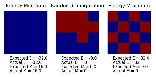
TASK: Run the ILcheck.py script from the IPython Qt console using the command ILcheck.py. The displayed window has a series of control buttons in the bottom left, one of which will allow you to export the figure as a PNG image. Save an image of the ILcheck.py output, and include it in your report.

TASK: How many configurations are available to a system with 100 spins? To evaluate these expressions, we have to calculate the energy and magnetisation for each of these configurations, then perform the sum. Let's be very, very, generous, and say that we can analyse $1\times 10^9$ configurations per second with our computer. How long will it take to evaluate a single value of ${⟨M⟩}_T$?

There are $2^{100}$ configurations in a system with 100 spins. Therefore it would take $2^{100}÷10^9\approx 1.27\times 10^{21}s$.

JC: Correct, but can you express it in more intuitive units, e.g. years?

TASK: Implement a single cycle of the above algorithm in the montecarlocycle(T) function. This function should return the energy of your lattice and the magnetisation at the end of the cycle. You may assume that the energy returned by your energy() function is in units of $k_B$! Complete the statistics() function. This should return the following quantities whenever it is called: $<E>,<E^2>,<M>,<M^2>$, and the number of Monte Carlo steps that have elapsed.

def montecarlostep(self, T):
        #this function performs a single Monte Carlo step
	energy_original = self.energy()
	lattice_old = self.lattice
		
        #the following two lines will select the coordinates of the random spin for you
	random_i = np.random.choice(range(0, self.n_rows))
	random_j = np.random.choice(range(0, self.n_cols))
		
	#changing the spin of selected cell
	self.lattice[random_i][random_j] *= -1
	energy_new = self.energy()
	#calculating energy change
	energy_change = energy_new - energy_original
		
	#checking if energy change is positive
	if energy_change > 0:				
		#the following line will choose a random number in the range [0,1) for you
		random_number = np.random.random()
		
		#determining whether or not to accept new configuration
		if random_number > np.exp(-1 * energy_change / T):
			#reverting to original configuration
			self.lattice[random_i][random_j] *= -1			
			self.E += energy_original
			self.E2 += energy_original ** 2
		else:
			self.E += energy_new
			self.E2 += energy_new ** 2
	else:
		self.E += energy_new
		self.E2 += energy_new ** 2
		
	magnetisation = self.magnetisation()
	self.M += magnetisation
	self.M2 += magnetisation ** 2
	
	self.n_cycles += 1
	
	return self.energy(),self.magnetisation()

def statistics(self):
	#This function returns the average values of E, E^2, M, M^2 and the number of monte carlo cyles
	step_number = self.n_cycles
	E_avg = self.E / step_number
	E2_avg = self.E2 / step_number
	M_avg = self.M / step_number
	M2_avg = self.M2 / step_number
	
	return E_avg,E2_avg,M_avg,M2_avg

JC: Code is clearly laid out and annotated with comments.

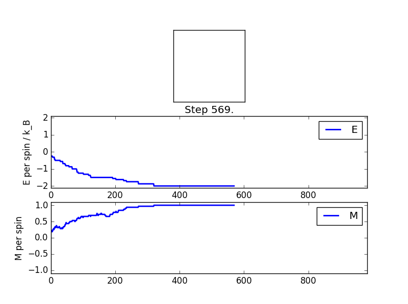
TASK: If $T<T_C$, do you expect a spontaneous magnetisation (i.e. do you expect $⟨M⟩\ne 0$)? When the state of the simulation appears to stop changing (when you have reached an equilibrium state), use the controls to export the output to PNG and attach this to your report. You should also include the output from your statistics() function.

Statistics function output:

TASK: Use the script ILtimetrial.py to record how long your current version of IsingLattice.py takes to perform 2000 Monte Carlo steps. This will vary, depending on what else the computer happens to be doing, so perform repeats and report the error in your average!

$mean=(5.458+5.407+5.399+5.400+5.405)÷5=5.414s(4sf)$

$STD=\sqrt{((5.458^2+5.407^2+5.399^2+5.400^2+5.405^2)÷5-5.4138^2)}=0.022s$

TASK: Look at the documentation for the NumPy sum function. You should be able to modify your magnetisation() function so that it uses this to evaluate M. The energy is a little trickier. Familiarise yourself with the NumPy roll and multiply functions, and use these to replace your energy double loop (you will need to call roll and multiply twice!).

def energy(self):
	energy = 0		
		
	lattice_shift_right = np.roll(self.lattice, -1, axis = 1)
	lattice_shift_down = np.roll(self.lattice, -1, axis = 0)
	new_lattice = np.multiply(self.lattice,lattice_shift_right) + np.multiply(self.lattice,lattice_shift_down)
	energy = -1 * np.sum(new_lattice)
		
	return energy

def magnetisation(self):		
	magnetisation = np.sum(self.lattice)
		
	return magnetisation

JC: Well noticed that you only need to use roll twice, rather than 4 times, if you remove the fact of 1/2 from the energy.

TASK: Use the script ILtimetrial.py to record how long your new version of IsingLattice.py takes to perform 2000 Monte Carlo steps. This will vary, depending on what else the computer happens to be doing, so perform repeats and report the error in your average!

$mean=(0.182+0.182+0.181+0.181+0.181)÷5=0.181s(3sf)$

$STD=\sqrt{((0.182^2+0.182^2+0.181^2+0.181^2+0.181^2)÷5-0.1814^2)}=0.0005s$

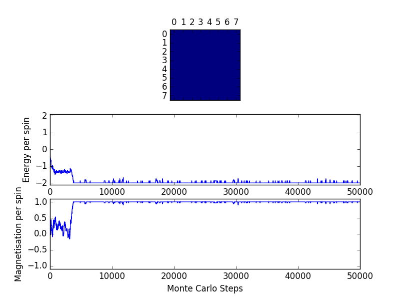
TASK: The script ILfinalframe.py runs for a given number of cycles at a given temperature, then plots a depiction of the final lattice state as well as graphs of the energy and magnetisation as a function of cycle number. This is much quicker than animating every frame! Experiment with different temperature and lattice sizes. How many cycles are typically needed for the system to go from its random starting position to the equilibrium state? Modify your statistics() and montecarlostep() functions so that the first N cycles of the simulation are ignored when calculating the averages. You should state in your report what period you chose to ignore, and include graphs from ILfinalframe.py to illustrate your motivation in choosing this figure.

The image below shows that an 8x8 lattice took around 4000 cycles to reach equilibrium, therefore I decided to ignore the first 5000 cycles when calculating averages.

JC: Did you look at other systems and other temperatures? Is this enough steps for the larger systems or systems at other temperatures to equilibrate?

def montecarlostep(self, T):
        # complete this function so that it performs a single Monte Carlo step
	energy_original = self.energy()
	lattice_old = self.lattice
		
        #the following two lines will select the coordinates of the random spin for you
	random_i = np.random.choice(range(0, self.n_rows))
	random_j = np.random.choice(range(0, self.n_cols))
		
	#changing the spin of selected cell
	self.lattice[random_i][random_j] *= -1
	energy_new = self.energy()
	#calculating energy change
	energy_change = energy_new - energy_original
		
	#checking if energy change is positive
	if energy_change > 0:				
		#the following line will choose a random number in the range [0,1) for you
		random_number = np.random.random()
			
		#determining whether or not to accept new configuration
		if random_number > np.exp(-1 * energy_change / T):
			#reverting to original configuration
			self.lattice[random_i][random_j] *= -1
				
			#only record energy after 5000 cycles
			if self.n_cycles >= 5000:
				self.E += energy_original
				self.E2 += energy_original ** 2
		elif self.n_cycles >= 5000:
			self.E += energy_new
			self.E2 += energy_new ** 2
	elif self.n_cycles >= 5000:
		self.E += energy_new
		self.E2 += energy_new ** 2
		
	magnetisation = self.magnetisation()
	
	#only record magnetisation after 5000 cycles 
	if self.n_cycles >= 5000:
		self.M += magnetisation
		self.M2 += magnetisation ** 2
	
	self.n_cycles += 1
	
	return self.energy(),self.magnetisation()

def statistics(self):
	#This function returns the average values of E, E^2, M, M^2 and the number of monte carlo cyles
	step_number = self.n_cycles - 5000
	E_avg = self.E / step_number
	E2_avg = self.E2 / step_number
	M_avg = self.M / step_number
	M2_avg = self.M2 / step_number
		
	return E_avg,E2_avg,M_avg,M2_avg,step_number

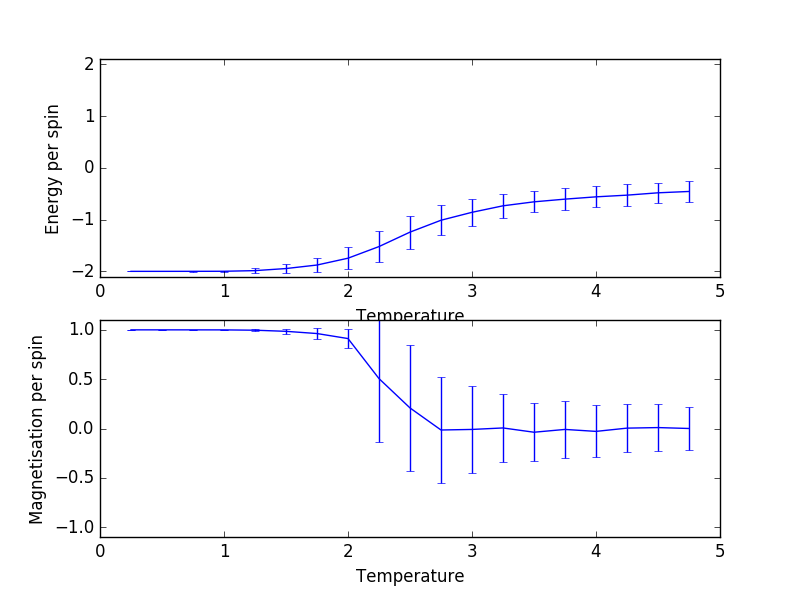
TASK: Use ILtemperaturerange.py to plot the average energy and magnetisation for each temperature, with error bars, for an $8\times 8$ lattice. Use your initution and results from the script ILfinalframe.py to estimate how many cycles each simulation should be. The temperature range 0.25 to 5.0 is sufficient. Use as many temperature points as you feel necessary to illustrate the trend, but do not use a temperature spacing larger than 0.5. T NumPy function savetxt() stores your array of output data on disk — you will need it later. Save the file as 8x8.dat so that you know which lattice size it came from.

The figure below was created using temperature range of 0.25 to 5 with a temperaure spacing of 0.25 and 100000 monte carlo cycles were done for each temperature.

TASK: Repeat the final task of the previous section for the following lattice sizes: 2x2, 4x4, 8x8, 16x16, 32x32. Make sure that you name each datafile that your produce after the corresponding lattice size! Write a Python script to make a plot showing the energy per spin versus temperature for each of your lattice sizes. Hint: the NumPy loadtxt function is the reverse of the savetxt function, and can be used to read your previously saved files into the script. Repeat this for the magnetisation. As before, use the plot controls to save your a PNG image of your plot and attach this to the report. How big a lattice do you think is big enough to capture the long range fluctuations?

From the figure below it can be seen that a lattice size of at least 16x16 is required to capture long range fluctuations.

TASK: By definition,

$C=\frac{\partial ⟨E⟩}{\partial T}$

From this, show that

$C=\frac{\mathrm{V}\mathrm{a}\mathrm{r}[E]}{k_B{T}^2}$

$⟨E⟩=\frac{\sum _i{E}_i{e}^{\frac{-E_i}{k_{B}T}}}{\sum _i{e}^{\frac{-E_i}{k_{B}T}}}$

$\frac{\partial ⟨E⟩}{\partial T}=\frac{(\sum _i\frac{{E_i}^2}{k_B{T}^2}{e}^{\frac{-E_i}{k_{B}T}})(\sum _i{e}^{\frac{-E_i}{k_{B}T}})-(\sum _i\frac{E_i}{k_B{T}^2}{e}^{\frac{-E_i}{k_{B}T}})(\sum _i{E}_i{e}^{\frac{-E_i}{k_{B}T}})}{(\sum _i{e}^{\frac{-E_i}{k_{B}T}}{)}^2}$

$=\frac{1}{k_B{T}^2}(\frac{\sum _i{E_i}^2{e}^{\frac{-E_i}{k_{B}T}}}{\sum _i{e}^{\frac{-E_i}{k_{B}T}}}-{\left(\frac{\sum _i{E}_i{e}^{\frac{-E_i}{k_{B}T}}}{\sum _i{e}^{\frac{-E_i}{k_{B}T}}}\right)}^2)$

$=\frac{⟨E^2⟩-{⟨E⟩}^2}{k_B{T}^2}$

$=\frac{Var[E]}{k_B{T}^2}$

JC: Good clear derivation.

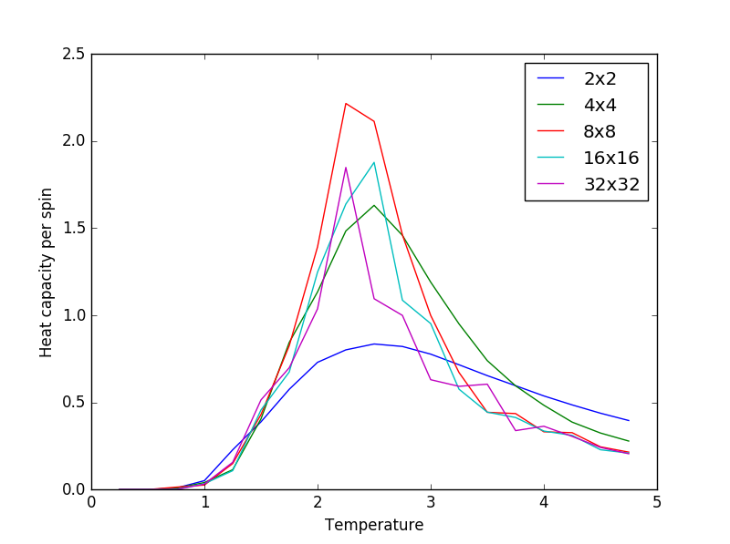
TASK: Write a Python script to make a plot showing the heat capacity versus temperature for each of your lattice sizes from the previous section. You may need to do some research to recall the connection between the variance of a variable, $\mathrm{V}\mathrm{a}\mathrm{r}[X]$, the mean of its square $⟨X^2⟩$, and its squared mean ${⟨X⟩}^2$. You may find that the data around the peak is very noisy — this is normal, and is a result of being in the critical region. As before, use the plot controls to save your a PNG image of your plot and attach this to the report.

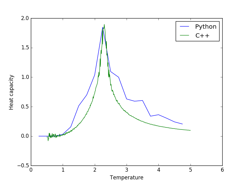
TASK: A C++ program has been used to run some much longer simulations than would be possible on the college computers in Python. You can view its source code here if you are interested. Each file contains six columns: $T,E,E^2,M,M^2,C$ (the final five quantities are per spin), and you can read them with the NumPy loadtxt function as before. For each lattice size, plot the C++ data against your data. For one lattice size, save a PNG of this comparison and add it to your report — add a legend to the graph to label which is which. To do this, you will need to pass the label="..." keyword to the plot function, then call the legend() function of the axis object (documentation here).

Lattice size used in the figure below was 32x32.

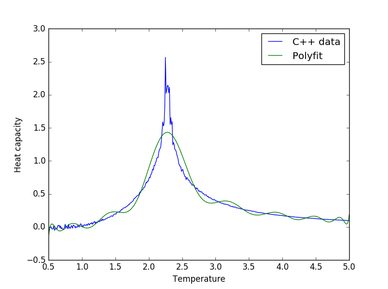
TASK: write a script to read the data from a particular file, and plot C vs T, as well as a fitted polynomial. Try changing the degree of the polynomial to improve the fit — in general, it might be difficult to get a good fit! Attach a PNG of an example fit to your report.

The figure below shows the C++ data for the 64 by 64 system and a degree of 20 was used for polyfit.

from IsingLattice import *
from matplotlib import pylab as pl
import numpy as np

lattice_size = "64"
file_name = "C++_data/" + lattice_size + "x" + lattice_size + ".dat"
data = np.loadtxt(file_name)
T = data[:,0]
C = []

for i in range(len(data)):
	C.append(data[i][5])

T_min = np.min(T)
T_max = np.max(T)

fit = np.polyfit(T, C, 20)
T_range = np.linspace(T_min, T_max, 1000) #generate 1000 evenly spaced points between T_min and T_max
fitted_c_values = np.polyval(fit, T_range) # use the fit object to generate the corresponding values of C

fig = pl.figure()
graph = fig.add_subplot(1,1,1)
graph.set_ylabel("Heat capacity")
graph.set_xlabel("Temperature")
graph.plot(T, C, label = "C++ data")
graph.plot(T_range, fitted_c_values, label = "Fitted data")
graph.legend(['C++ data','Polyfit'])
pl.show()

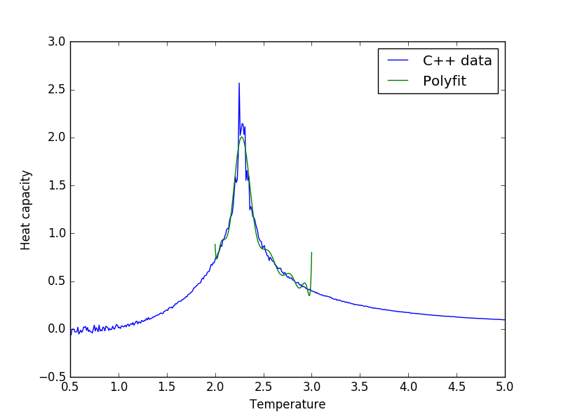
TASK: Modify your script from the previous section. You should still plot the whole temperature range, but fit the polynomial only to the peak of the heat capacity! You should find it easier to get a good fit when restricted to this region.

The figure below shows the C++ data for the 64 by 64 system and a degree of 20 was used for polyfit and polyfit was only applied to between T=2 and T=3.

from IsingLattice import *
from matplotlib import pylab as pl
import numpy as np

lattice_size = "64"
file_name = "C++_data/" + lattice_size + "x" + lattice_size + ".dat"
data = np.loadtxt(file_name)
T = data[:,0]
C = []

for i in range(len(data)):
	C.append(data[i][5])

C = np.asarray(C)
T_min = 2
T_max = 3
selection = np.logical_and(T > T_min, T < T_max) #choose only those rows where both conditions are true
peak_T_values = T[selection]
peak_C_values = C[selection]

fit = np.polyfit(peak_T_values, peak_C_values, 20)
T_range = np.linspace(T_min, T_max, 1000) #generate 1000 evenly spaced points between T_min and T_max
fitted_c_values = np.polyval(fit, T_range) # use the fit object to generate the corresponding values of C

fig = pl.figure()
graph = fig.add_subplot(1,1,1)
graph.set_ylabel("Heat capacity")
graph.set_xlabel("Temperature")
graph.plot(T, C, label = "C++ data")
graph.plot(T_range, fitted_c_values, label = "Fitted data")
graph.legend(['C++ data','Polyfit'])
pl.show()

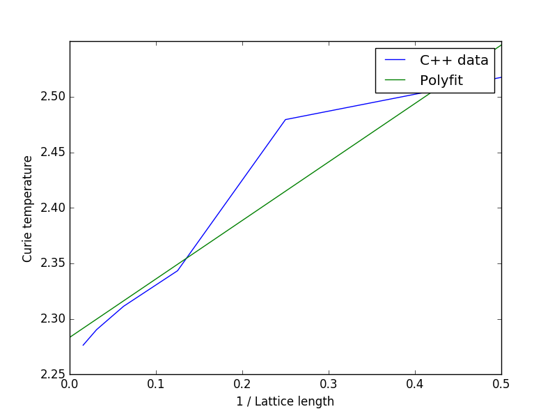
TASK: find the temperature at which the maximum in C occurs for each datafile that you were given. Make a text file containing two colums: the lattice side length (2,4,8, etc.), and the temperature at which C is a maximum. This is your estimate of $T_C$ for that side length. Make a plot that uses the scaling relation given above to determine $T_{C,\mathrm{\infty }}$. By doing a little research online, you should be able to find the theoretical exact Curie temperature for the infinite 2D Ising lattice. How does your value compare to this? Are you surprised by how good/bad the agreement is? Attach a PNG of this final graph to your report, and discuss briefly what you think the major sources of error are in your estimate.

The figure below shows that $T_{C,\mathrm{\infty }}$ for a 2D lattice is around 2.285, the theoretical Curie temperature for the infinite 2D Ising lattice is 2.269(4sf), according to http://www.nyu.edu/classes/tuckerman/stat.mech/lectures/lecture_26/node2.html [accessed on 17/11/2016]. This value is very close to the value predicted using the C++ data. The major sources of error would have been caused by the fact that data from the 2x2, 4x4, and 8x8 lattice were used to estimate the $T_{C,\mathrm{\infty }}$, this is because my figures from one of the previous tasks showed that only systems with lattice size of 16x16 and above should be used to predict long range fluctuations.

JC: What about removing the 2x2 system from your fit since that gives an especially bad description of an infinite lattice since every spin only has 2 different neighbouring spins.