Talk:Mod:paxtonchia250893
JC: General comments: Good report with clearly written answers to all tasks. You could add a bit more detail to some of your discussions of your own results though and use the background theory to the experiment to support your explanations.
Introduction to molecular dynamics simulation
Velocity Verlet Algorithm
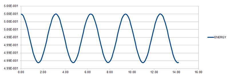
By using the data and formulas given in HO.xls, the three columns "ANALYTICAL", "ERROR", and "ENERGY" were completed. ANALYTICAL was filled in using the formula for the classical harmonic oscillator . ERROR was determined by the absolute difference between the ANALYTICAL and the velocity-Verlet solution while ENERGY is calculated by adding up both potential and kinetic energy of the harmonic oscillator. The formula for ENERGY is given by . The graphs of the three variables with respect to time are shown below.
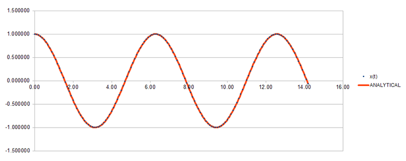
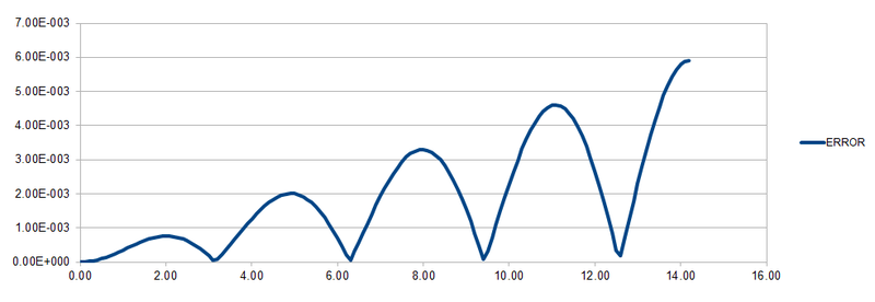
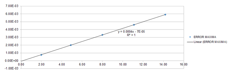
For the default timestep, the positions of the maxima are estimated at t = 2.00, 4.90, 8.00, 11.10 and 14.20. These points are plotted against time and a linear function is fitted to the data as shown below.
Different timesteps are experimented and the maximum change in energy is plotted as a percentage against time.
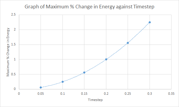
As shown in the above graph, as the timestep increases, the change in energy also increases. Hence, a small timestep (≤0.200) is required to ensure that the total energy does not change by more than 1% over the course of the simulation. It is important to monitor the total energy of a physical system when modelling its behaviour numerically to ensure that the error in calculating the properties of the system are not large.
JC: Good thorough analysis of the timestep, why does the error oscillate? Energy should be conserved so we need to make sure this is approximately true in our simulations.
Single Lennard-Jones Interaction
Working with a single Lennard-Jones interaction, was substituted into the equation to find the separation, , at which the potential energy is zero. The results obtained are as follows:
The force at this separation, , can be calculated using the formula .
Substitute
The equilibrium separation, , occurs when the force, , is zero.
The well-depth, , is calculated as follows:
When , .
JC: All maths correct and well laid out.
Periodic Boundary Conditions
To estimate the number of water molecules given a volume under standard conditions, the following equation can be used:
Similarly, the equation can be rearranged to find the volume of water given the number of molecules under standard conditions.
Hence, realistic volumes of liquid cannot be simulated and periodic boundary conditions are used. This can be illustrated in the following example. An atom at position in a cubic simulation box which runs from to . In a single timestep, it moves along the vector . The atom's end point before applying the periodic boundary conditions can be found by adding the vector to the atom's original position, which gives us . Since the box has the dimensions , any value in the end position that is larger than 1 will have 1 subtracted from it after applying the periodic boundary conditions, resulting in as the end point.
Reduced Units
By rearranging the equations given,
JC: All calculations correct.
Equilibration
Simulation Box
Generating a random position for each atom to create a simulation box can cause problems in simulations if the atoms are generated close together. This results in a large repulsion between the atoms and may cause the atoms to move too far and out of range in a single timestep.
JC: This can make the simulation crash.
With a lattice spacing in x,y,z = 1.07722 1.07722 1.07722, the volume of the unit cell is 1.077223 = 1.25. Since there is one lattice point per unit cell in a simple cubic lattice, the number of lattice points per unit volume (number density) corresponds to .
For a face-centred cubic lattice, there are 4 lattice points per unit cell. With a lattice point density of 1.2, the volume of the unit cell is . Hence, the length of the unit cell is .
If a face-centred cubic lattice was used instead, 4000 atoms will be created as there are 4 lattice points per unit cell and the box contains 1000 unit cells.
JC: Correct.
Properties of Atoms
The purpose of the following commands in the input script are found from the LAMMPS manual[1] as follows:
"mass 1 1.0" sets the mass for all atoms of type 1 to 1.0.
"pair_style lj/cut 3.0" tells LAMMPS to use the standard 12/6 Lennard-Jones potential between the atoms with a cutoff of 3.0 when calculating the forces. This means that the interaction between a pair of atoms is only calculated if their separation is less than 3.0.
"pair_coeff * * 1.0 1.0" sets both the parameters of the Lennard-Jones potential, and , to 1.0 for atom pairs of any type.
If we are specifying the initial position and velocity, we are going to use the velocity verlet algorithm.
JC: Good, why is a cutoff used for this potential?
Running the Simulation
The purpose of assigning a value to a text variable (e.g. timestep or n_steps) is for our own convenience. If we need to change the value of the variable, we only need to change the value assigned to the text variable. This only requires us to make a single edit instead of having to change the value every time it is used in the code.
Checking Equilibration
The thermodynamics output of the first simulations were analysed to see how long it takes to reach an equilibrium state. Graphs of energy, temperature and pressure against time for the 0.001 timestep experiment are shown below:

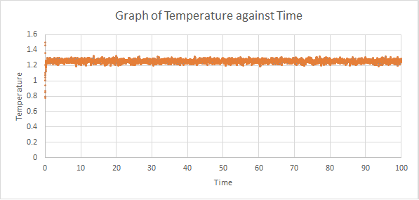
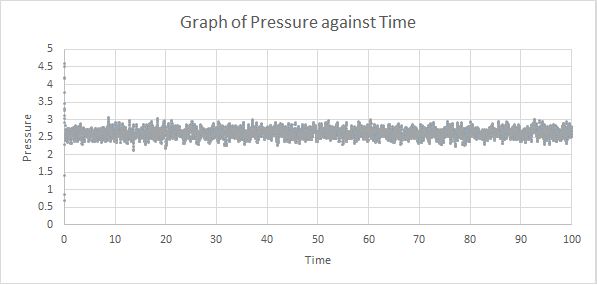
As shown above, all three thermodynamic output reached a constant average within the simulation time, which meant that an equilibrium state was reached. From the graph of energy against time, the system reached equilibrium at around t = 0.4.
A single graph of energy against time for all timesteps is plotted as shown:

A timestep of 0.0025 is the largest to give acceptable results as larger timesteps give energies that are higher than that using a timestep of 0.001. Using a timestep of 0.015 is particularly bad because the system did not reach an equilibrium state.
JC: Good choice of timestep, the average total energy shouldn't depend on the choice of timestep so all timesteps above 0.0025 are no good. Choose the largest of the acceptable timesteps - 0.0025 - to allow the simulation to cover as much time as possible.
Running simulations under specific conditions
Thermostats and Barostats
Temperature is controlled by multiplying every velocity by a constant factor , which can be evaluated as follows, starting from the given equation:
JC: Correct.
Examining the Input Script
fix aves all ave/time 100 1000 100000 v_dens v_temp v_press v_dens2 v_temp2 v_press2
run 100000
For the above line in the input script, "100" means that input values are used every 100 timesteps. "1000" means that 1000 input values are used to calculate the averages. "100000" means that averages are calculated every 100000 timesteps.[1] Values of each variable e.g. temperature will be sampled every 100 timesteps and 1000 measurements contribute to the average. The simulation will run for 100000 timesteps. With a timestep of 0.0025, 250 time units will be simulated.
Plotting the Equations of State
10 constant pressure/temperature simulations were ran with 5 different temperatures (T = 2, 3, 4, 5, 6) each at 2 different pressures (P = 2, 3). The value of the timestep chosen was 0.0025. Graphs of density against temperature were plotted separately for the 2 pressures. Error bars in both x and y directions and a line corresponding to the density predicted by the ideal gas law were included. As and are both 1.0, the ideal gas equation expressed in reduced units is .
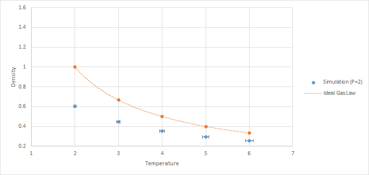
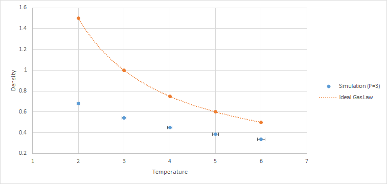
The simulated density is lower than the ideal gas density for both pressures. This is due to the approximation used in the ideal gas law, where there are no repulsive forces between the particles. However, in the simulation, the atoms are modeled using the Lennard-Jones potential, which accounts for the repulsion between atoms. This causes the atoms in the simulation to be further apart from one another when compared to the ideal gas under the same conditions. Hence, the density of the simulated liquid is lower than the ideal gas.
As pressure increases, the discrepancy increases. This is due to higher pressures causing the atoms to be closer to one another. Hence, the repulsion forces between the atoms in the simulation increases, resulting in larger deviations from the ideal gas.
JC: Good, plot results on a single graph to show the trend with pressure more clearly, what about the trend with temperature? The ideal gas is a good approximation to low density gases, where interparticle interactions are less significant.
Calculating heat capacities using statistical physics
10 constant volume/temperature simulations were ran with 5 different temperatures (T = 2.0, 2.2, 2.4, 2.6, 2.8) each at 2 different densities (0.2 and 0.8). A graph of was plotted against .
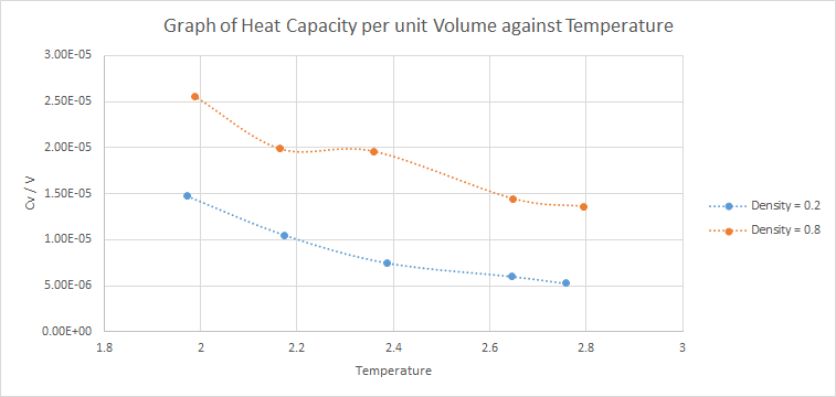
The expected trend is that heat capacity decreases with temperature, which is the trend shown in the graph above. Heat capacity measures the amount of energy required to increase the temperature of the system. As temperature increases, the vibrational energy levels of the system are more accessible and lesser energy will be required to increase the temperature of the system. Hence, heat capacity decreases as temperature increases.
Furthermore, a larger density means that there are more atoms per unit volume. Since heat capacity is an extensive property, is higher for the simulation with larger density. However, one would expect to be proportional to density but the heat capacity for is not 4 times as large as that for .
JC: You are simulating a system of spherical particles so there are no vibrational energy levels, but the heat capacity can be related to the density of energy levels (density of states since the system is classical).
An example of my input script is included as follows:
### SPECIFY THE REQUIRED THERMODYNAMIC STATE ###
variable d equal 0.2
variable T equal 2.0
variable timestep equal 0.0025

### DEFINE SIMULATION BOX GEOMETRY ###
lattice sc ${d}
region box block 0 15 0 15 0 15
create_box 1 box
create_atoms 1 box

### DEFINE PHYSICAL PROPERTIES OF ATOMS ###
mass 1 1.0
pair_style lj/cut/opt 3.0
pair_coeff 1 1 1.0 1.0
neighbor 2.0 bin

### ASSIGN ATOMIC VELOCITIES ###
velocity all create ${T} 12345 dist gaussian rot yes mom yes

### SPECIFY ENSEMBLE ###
timestep ${timestep}
fix nve all nve

### THERMODYNAMIC OUTPUT CONTROL ###
thermo_style custom time etotal temp press
thermo 10

### RECORD TRAJECTORY ###
dump traj all custom 1000 output-1 id x y z

### RUN SIMULATION TO MELT CRYSTAL ###
run 10000
unfix nve
reset_timestep 0

### BRING SYSTEM TO REQUIRED STATE ###
variable tdamp equal ${timestep}*100
fix nvt all nvt temp ${T} ${T} ${tdamp}
run 10000
reset_timestep 0

###SWITCH OFF THERMOSTAT###
unfix nvt
fix nve all nve

### MEASURE SYSTEM STATE ###
thermo_style custom step etotal temp press density vol atoms
variable dens equal density
variable temp equal temp
variable temp2 equal temp*temp
variable press equal press
variable atoms equal atoms
variable etotal equal etotal
variable etotal2 equal etotal*etotal
variable vol equal vol
fix aves all ave/time 100 1000 100000 v_dens v_temp v_press v_etotal v_etotal2 v_temp2
run 100000

variable avedens equal f_aves[1]
variable avetemp equal f_aves[2]
variable avepress equal f_aves[3]
variable aveetotal equal f_aves[4]
variable aveetotal2 equal f_aves[5]
variable heatcap equal ${atoms}*${atoms}*(f_aves[5]-f_aves[4]*f_aves[4])/f_aves[6]

print "Averages"
print "--------"
print "Number of atoms: ${atoms}"
print "Volume: ${vol}"
print "Energy: ${aveetotal}"
print "Energy2: ${aveetotal2}"
print "Heat Capacity: ${heatcap}"
print "Density: ${avedens}"
print "Temperature: ${avetemp}"
print "Pressure: ${avepress}"
Structural properties and the radial distribution function
The simulations of the Lennard-Jones system were ran for three phases using the values shown in the table below[2] and the RDFs for the three systems are plotted.
| Phase | Density | Temperature |
|---|---|---|
| Vapour | 0.1 | 1.2 |
| Liquid | 0.8 | 1.2 |
| Solid | 1.2 | 1.2 |

The solid phase RDF has the most number of peaks and the peaks are present even at long distances. The liquid phase RDF has a few peaks that are only present at short distances. The vapour phase RDF has only one broad peak and decays the fastest to a constant of one. This is due to the solid phase having long range order where atoms are arranged in a well-defined manner for long distances while the liquid phase only has short range order where nearby atoms are ordered. The vapour phase is the most disordered with no apparent regular arrangement of the atoms.

The first three peaks of the solid phase RDF corresponds to the position of the nearest neighbour, second nearest neighbour and third nearest neighbour respectively. The diagram above shows the positions of these three nearest neighbour with respect to the lattice site in yellow. The lattice site in red is the nearest neighbour, while the lattice site in blue is the second nearest neighbour and the lattice site in green is the third nearest neighbour.
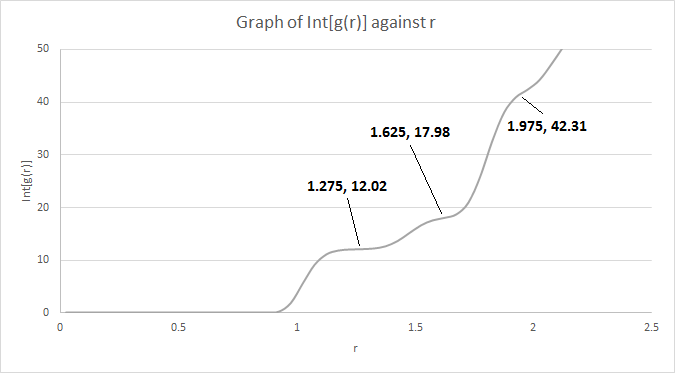
The lattice spacing is the distance of the second nearest neighbour, which is 1.475 as shown in the graph above. This also corresponds to the theoretical value calculated above (1.49380) for a FCC lattice with a lattice point density of 1.2. The coordination number for each of the three peaks can be obtained from the integrals of the peaks as shown above. The coordination number of the first peak is 12. As the graph shows a running integral, the coordination number of the second peak is 17.98 - 12.02 ≈ 6 while the coordination number of the third peak is 42.31 - 17.98 ≈ 24.
JC: Nice diagram to show which atoms are responsible for the first three peaks, do the coordination numbers that you've got from the integral of g(r) make sense based on the fcc structure? Could you have calculated the lattice parameter from each of the first three peaks separately, by expressing the distances to these atoms in terms of the lattice parameter using the geometry of an fcc lattice, and then calculated an average rather than just giving the value from the second peak?
Dynamical properties and the diffusion coefficient
Mean Squared Displacement
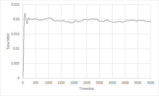
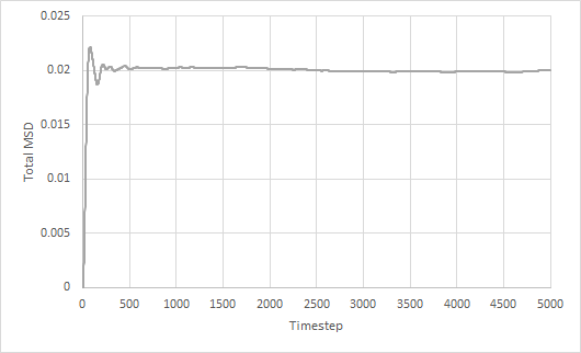
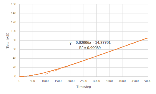
Mean squared displacement of solid, liquid and gas simulations as a function of timestep are plotted. The diffusion coefficient is estimated from the gradient of the total MSD against timestep graph.
The trend in the MSD graphs are as expected. The total MSD for the solid simulation stays approximately constant at 0.02 as the solid atoms are fixed in their lattice positions. This is also seen from its negligible diffusion coefficient. The total MSD for both liquid and gas increases linearly with time. However, the total MSD for gas increases much faster than that for liquid, which is also reflected in the larger diffusion coefficient. This is due to the gaseous atoms having weaker intermolecular forces between each other and being able to move more freely than liquid atoms.
For the large system, the trends in the MSD graphs are similar to that for a small system except for the gas phase. For solid and liquid, the MSD graphs and diffusion coefficients are approximately the same in both the large and small system. However, the total MSD for solid showed lesser fluctuations in the large system. On the other hand, the total MSD for gas increases much faster in the large system than the small system, which results in a larger diffusion coefficient as well.
JC: Why do you divide by 0.002 when you calculate the diffusion coefficient? Why is the gas MSD curved initially (ballistic motion), before eventually becoming linear?
Velocity Autocorrelation Function
The normalised velocity autocorrelation function for a 1D harmonic oscillator is evaluated as followsː
JC: Correct answer, but the integration in the last step of your derivation is not correct. The function sin(x)*cos(x) is an odd function (odd*even=odd) and so the integral of this function with limits which are symmetric about zero will be zero.
The velocity autocorrelation function of the 1D harmonic oscillator, solid simulation and liquid simulation were plotted as shown below.
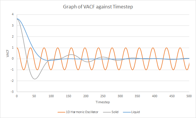
The minima in the VACFs for the liquid and solid system represent a reverse in the velocities of the atoms. In the solid system, the atoms vibrate about their fixed lattice positions and the interactions between neighbouring atoms disrupt this perfect oscillatory motion. Hence, the velocities of the solid system is not perfectly correlated to its initial velocity and the VACF for the solid system follows a damped oscillation. In the liquid system, the liquid atoms are free to move around so any oscillatory motion is rapidly disrupted by the diffusion of the liquid atoms. This results in the VACF for the liquid system to decay much faster to zero than the VACF for the solid system.[3] The harmonic oscillator VACF represents a perfect vibration where there are no interactions to disrupt the oscillatory motion. Its velocity reverses at the end of each oscillation and it does not decay after each oscillation. Therefore, the velocity is always correlated to its initial velocity and its VACF does not decay to zero, unlike the Lennard-Jones solid and liquid.
JC: Good, collisions between particles randomise particle velocities and cause the VACF to decay. The liquid does have a small minima before it becomes decorrelated.
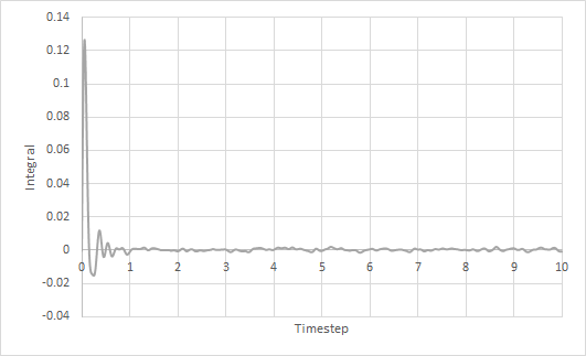
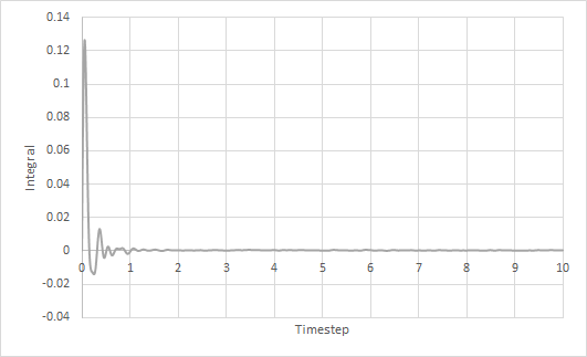
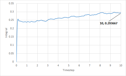
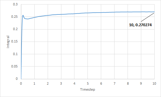
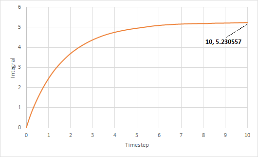
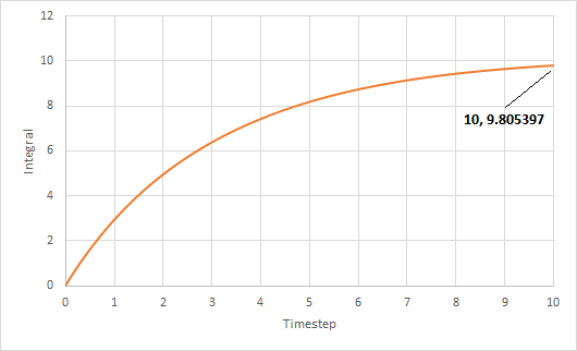
The trapezium rule was used to approximate the integral under the VACF for solid, liquid and gas. The graph of running integral against time is plotted as shown and the diffusion coefficient is estimated using the values of the integral at t = 10.
The diffusion coefficient of the solid system is approximately zero and increases from liquid to gas. Furthermore, using both VACF and MSD to calculate diffusion coefficients yield similar results, which is expected.
The largest source of error is probably not simulating a large enough amount of time for to reach zero. The simulation is only ran until and it can be seen from the running integral graphs that the integrals for the liquid and gas systems are still increasing. This means that the diffusion coefficients should be larger than my estimates.
JC: Good, using the trapezium rule for the integration also introduces some error.
References
- ↑ 1.0 1.1 LAMMPS Manual, http://lammps.sandia.gov/doc/Section_commands.html#cmd_5. Accessed on 17 Feb 2017.
- ↑ J. Hansen and L. Verlet, Phase Transitions of the Lennard-Jones System, Phys. Rev., 1969, 184, 151.DOI:10.1103/PhysRev.184.151
- ↑ The Velocity Autocorrelation Function, http://www.compsoc.man.ac.uk/~lucky/Democritus/Theory/vaf.html. Accessed 22 Feb 2017.
