Talk:Mod:mp1614LS

Molecular Dynamics Simulations of Simple Liquids

Nice report, you've covered all the points required and provide explanation with clarity. However, in some places (like the VACF discussion) you could go a bit further into theory. However, you had very nice explanations for the Cv trend and for ideal gas v. simulation. Nicely done - Mark 75/100

Introduction

Computer simulation is a powerful technique for studying systems, as in certain cases, it may not be possible to run a practical experiment due to factors such as cost, time, or even due to the danger posed by running certain experiments. Simulations can circumvent all of these factors and allow for the study of such systems, providing us with useful information and insights into these areas, allowing for the development of models and theories. Molecular dynamics (MD) is one such simulation method with is used to study the movements of particles, such as atoms or molecules. The main principle of MD involves allowing particles in a set space to interact for a set amount of time to observe a dynamical evolution of the system. The most common iteration of MD is the one in which particle trajectories are determined by numerically solving Newton's equations of motion. Properties such as the forces between particles and their potential energies are calculated using interatomic potentials or force-fields. In a MD simulation, the macroscopic properties of a system is explored using microscopic simulations. The connection between microscopic simulations and macroscopic properties is made via statistical mechanics, which provides the equations that relate macroscopic properties to the distribution and motion of the atoms and molecules in the system.

The objective of this computational laboratory was to run and analyse a set of simulations on a simple liquid using a software package called Large-scale Atomic/Molecular Massively Parallel Simulator (LAMMPS), in order to calculate various properties such as the heat capacity, Radial Distribution Function, and the diffusion coefficient. The underlying mathematics along with the effects of changing simulation parameters such as the timestep was also investigated, in order to provide an understanding of how LAMMPS and simulations in general operate. Tick

Introduction to molecular dynamics simulation

TASK: Open the file HO.xls. In it, the velocity-Verlet algorithm is used to model the behaviour of a classical harmonic oscillator. Complete the three columns "ANALYTICAL", "ERROR", and "ENERGY": "ANALYTICAL" should contain the value of the classical solution for the position at time $t$, "ERROR" should contain the absolute difference between "ANALYTICAL" and the velocity-Verlet solution (i.e. ERROR should always be positive -- make sure you leave the half step rows blank!), and "ENERGY" should contain the total energy of the oscillator for the velocity-Verlet solution. Remember that the position of a classical harmonic oscillator is given by $x\left(t\right)=A\cos (\omega t+\varphi )$ (the values of $A$, $\omega$, and $\varphi$ are worked out for you in the sheet).

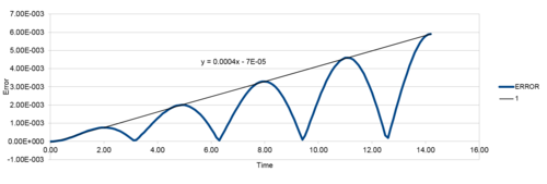
TASK: For the default timestep value, 0.1, estimate the positions of the maxima in the ERROR column as a function of time. Make a plot showing these values as a function of time, and fit an appropriate function to the data.

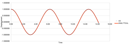
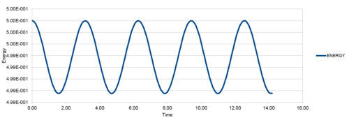
The graphs below show the change of displacement with time, change of energy with time, and calculated error between the classical solution and velocity-Verlet solution respectively.

The values for displacement given by the velocity-Verlet algorithm were compared to the values obtained from the classical harmonic oscillator. The position of the particle in the classical harmonic oscillator was given by $x\left(t\right)=A\cos (\omega t+\varphi )$. The error was calculated by subtracting the solution for the velocity-Verlet algorithm from the classical harmonic oscillator solution. For a classical harmonic oscillator, the total energy for the consists of two terms, the potential and kinetic energy, and was calculated using the formula $E=U+K$, where $U=\frac{1}{2}k{x}^2$ and $K=\frac{1}{2}m{v}^2$.

Displacement vs time for the velocity-Verlet algorithm	Total energy of the oscillator against time for the velocity-Verlet solution	The absolute error between the classical solution and the velocity-Verlet solution

Both the displacement and energy of the system show an oscillating relationship with time, with the displacement varying from 1 to -1, and the total energy oscillating around 0.4995. The error between the velocity-Verlet solution and classical solution can be seen to increase with time. The linear function that describes this error can be seen plotted on the graph.

TASK: Experiment with different values of the timestep. What sort of a timestep do you need to use to ensure that the total energy does not change by more than 1% over the course of your "simulation"? Why do you think it is important to monitor the total energy of a physical system when modelling its behaviour numerically?

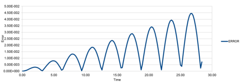
The graphs below show how the total energy and error change with time for a set of timesteps of 0.15, 0.2, and 0.25.

	Timestep
	0.15	0.2	0.25
Energy
Error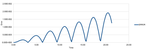

As the timestep was increased by increments of 0.05, the amplitude and frequency of the oscillation of the energy and hence the error was found to increase, due to a longer time between sampling of the system. The 2nd row in the table above shows the observed error for a range of timesteps. It can be seen that the total energy does not change by a more than 1% around a timestep of 0.2. When modelling a system numerically, it is important to monitor the total energy of a physical system when modelling its behaviour numerically as it must obey the law of conservation of energy, and if this law is not obeyed, it would indicate that something is wrong with the simulation. Additionally, monitoring the total energy allows for the opportunity to identify whether a system has equilibrated or not. If the energy has not reached equilibrium, it would be a strong indicator that there is a error somewhere. Tick, correct

TASK: For a single Lennard-Jones interaction, $\varphi \left(r\right)=4ϵ(\frac{{\sigma }^{12}}{r^{12}}-\frac{{\sigma }^6}{r^6})$, find the separation, $r_0$, at which the potential energy is zero. What is the force at this separation? Find the equilibrium separation, $r_{eq}$, and work out the well depth ($\varphi \left(r_{eq}\right)$). Evaluate the integrals $\underset{2\sigma }{\overset{\mathrm{\infty }}{\int }}\varphi \left(r\right)\mathrm{d}r$, $\underset{2.5\sigma }{\overset{\mathrm{\infty }}{\int }}\varphi \left(r\right)\mathrm{d}r$, and $\underset{3\sigma }{\overset{\mathrm{\infty }}{\int }}\varphi \left(r\right)\mathrm{d}r$ when $\sigma =ϵ=1.0$.

Find the separation, $r_0$, at which the potential energy is zero	Force at this separation	Find the equilibrium separation, $r_{eq}$	Work out the well depth ($\varphi \left(r_{eq}\right)$)
$\varphi \left(r_0\right)=0=4ϵ(\frac{{\sigma }^{12}}{{r_0}^{12}}-\frac{{\sigma }^6}{{r_0}^6})$ $0=\frac{{\sigma }^{12}}{{r_0}^{12}}-\frac{{\sigma }^6}{{r_0}^6}$ $\frac{{\sigma }^{12}}{{r_0}^{12}}=\frac{{\sigma }^6}{{r_0}^6}$ $\frac{{\sigma }^6}{{r_0}^6}=1$ ${\sigma }^6={r_0}^6$ $r_0=\sigma$ Tick	${\mathbf{F}}_i=-\frac{\mathrm{d}\varphi \left({\mathbf{r}}^N\right)}{\mathrm{d}{\mathbf{r}}_i}$ At $i=0$, $\varphi =0$ Therefore ${\mathbf{F}}_0=-\frac{\mathrm{d}\varphi \left({\mathbf{r}}^N\right)}{\mathrm{d}{\mathbf{r}}_0}$ ${\mathbf{F}}_0=-24ϵ(2\frac{{\sigma }^{12}}{{r_0}^{13}}-\frac{{\sigma }^6}{{r_0}^7})$ Using $r_0=\sigma$ gives ${\mathbf{F}}_0=\frac{24ϵ}{\sigma }$	$\frac{\mathrm{d}\varphi \left({\mathbf{r}}^N\right)}{\mathrm{d}{\mathbf{r}}_i}=0$ $24ϵ(2\frac{{\sigma }^{12}}{{r_i}^{13}}-\frac{{\sigma }^6}{{r_i}^7})=0$ $2\frac{{\sigma }^{12}}{{r_i}^{13}}=\frac{{\sigma }^6}{{r_i}^7}$ $\frac{2{\sigma }^6}{r_i}=1$ $r_{eq}=2^{1/6}\sigma$ Tick	$\varphi \left(r_{eq}\right)=4ϵ(\frac{{\sigma }^{12}}{{r_{eq}}^{12}}-\frac{{\sigma }^6}{{r_{eq}}^6})$ $r_{eq}=2^{1/6}\sigma$ $\varphi \left(r_{eq}\right)=4ϵ(\frac{{\sigma }^{12}}{(2^{1/6}\sigma {)}^{12}}-\frac{{\sigma }^6}{(2^{1/6}\sigma {)}^6})$ $\varphi \left(r_{eq}\right)=4ϵ(\frac{1}{4}-\frac{1}{2})$ $\varphi \left(r_{eq}\right)=4ϵ(-\frac{1}{4})$ $\varphi \left(r_{eq}\right)=-ϵ$ Tick
Evaluate $\underset{2\sigma }{\overset{\mathrm{\infty }}{\int }}\varphi \left(r\right)\mathrm{d}r$ when $\sigma =ϵ=1.0$	Evaluate $\underset{2.5\sigma }{\overset{\mathrm{\infty }}{\int }}\varphi \left(r\right)\mathrm{d}r$when $\sigma =ϵ=1.0$	Evaluate $\underset{3\sigma }{\overset{\mathrm{\infty }}{\int }}\varphi \left(r\right)\mathrm{d}r$ when $\sigma =ϵ=1.0$
$\underset{2\sigma }{\overset{\mathrm{\infty }}{\int }}4ϵ(\frac{{\sigma }^{12}}{r^{12}}-\frac{{\sigma }^6}{r^6})\mathrm{d}r$ $=4ϵ\underset{2\sigma }{\overset{\mathrm{\infty }}{\int }}(\frac{{\sigma }^{12}}{r^{12}}-\frac{{\sigma }^6}{r^6})\mathrm{d}r$ $=4ϵ{[-\frac{{\sigma }^{12}}{11r^{11}}+\frac{{\sigma }^6}{5r^5}]}_{2\sigma }^{\mathrm{\infty }}$ $=4ϵ(0)$ $-$ $4ϵ(-\frac{{\sigma }^{12}}{11(2\sigma {)}^{11}}+\frac{{\sigma }^6}{5(2\sigma {)}^5})$ $=0-$ $4(-\frac{1}{11(2{)}^{11}}+\frac{1}{5(2{)}^5})$ $=0-$ $0.02482244318$ $=-0.0248$ Tick	$\underset{2.5\sigma }{\overset{\mathrm{\infty }}{\int }}4ϵ(\frac{{\sigma }^{12}}{r^{12}}-\frac{{\sigma }^6}{r^6})\mathrm{d}r$ $=4ϵ\underset{2.5\sigma }{\overset{\mathrm{\infty }}{\int }}(\frac{{\sigma }^{12}}{r^{12}}-\frac{{\sigma }^6}{r^6})\mathrm{d}r$ $=4ϵ{[-\frac{{\sigma }^{12}}{11r^{11}}+\frac{{\sigma }^6}{5r^5}]}_{2.5\sigma }^{\mathrm{\infty }}\mathrm{d}r$ $=4ϵ(0)$ $-$ $4ϵ(-\frac{{\sigma }^{12}}{11(2.5\sigma {)}^{11}}+\frac{{\sigma }^6}{5(2.5\sigma {)}^5})$ $=0-$ $4(-\frac{1}{11(2.5{)}^{11}}+\frac{1}{5(2.5{)}^5})$ $=0-$ $0.008176747985$ $=-0.00818$ Tick	$\underset{3\sigma }{\overset{\mathrm{\infty }}{\int }}4ϵ(\frac{{\sigma }^{12}}{r^{12}}-\frac{{\sigma }^6}{r^6})\mathrm{d}r$ $=4ϵ\underset{3\sigma }{\overset{\mathrm{\infty }}{\int }}(\frac{{\sigma }^{12}}{r^{12}}-\frac{{\sigma }^6}{r^6})\mathrm{d}r$ $=4ϵ{[-\frac{{\sigma }^{12}}{11r^{11}}+\frac{{\sigma }^6}{5r^5}]}_{3\sigma }^{\mathrm{\infty }}\mathrm{d}r$ $=4ϵ(0)$ $-$ $4ϵ(-\frac{{\sigma }^{12}}{11(3\sigma {)}^{11}}+\frac{{\sigma }^6}{5(3\sigma {)}^5})$ $=0-$ $4(-\frac{1}{11(3{)}^{11}}+\frac{1}{5(3{)}^5})$ $=0-$ $0.003290128332$ $=-0.00329$ Tick, good

TASK: Estimate the number of water molecules in 1ml of water under standard conditions. Estimate the volume of $10000$ water molecules under standard conditions.

Number of water molecules in 1 ml	Volume of 10000 water molecules
${\rho }_{H_{2}O}=1gmo{l}^{-1}\approx 1g$ $M_{H_{2}O}\approx 18gmo{l}^{-1}$ $\frac{1}{18}=0.\dot{5}mol$ $N=moles\times N_A$ $N=0.\dot{5}\times (6.022\times 10^{23})$ $N=3.3\times 10^{22}molecules$ Tick	$\rho =\frac{m}{V}$, where $\rho$ = density, $m$= mass, and $V$ = volume. ${\rho }_{H_{2}O}=\frac{m_{H_{2}O}}{V}$ $1=\frac{(10000\times \frac{18}{6.023\times 10^{23}})}{V}$ $V=10000\times \frac{18}{6.022\times 10^{23}}$ $$\begin{gathered} V=2.99\times 10^{-19} \\ ml \end{gathered}$$ Tick

TASK: Consider an atom at position $(0.5,0.5,0.5)$ in a cubic simulation box which runs from $(0,0,0)$ to $(1,1,1)$. In a single timestep, it moves along the vector $(0.7,0.6,0.2)$. At what point does it end up, after the periodic boundary conditions have been applied?.

The application of periodic boundary conditions ensures that when an object such as an atom or molecule passes through one side of the simulation box, it re-appears on the opposite side, meaning that only of the properties of the original simulation box need to be tracked and recorded, rather than creating and tracking an increasing number of new boxes, which would be extremely expensive in terms of required computational power. In this case, the atom would end up at the point $(0.2,0.1,0.7)$ once the conditions have been applied. Tick

TASK: The Lennard-Jones parameters for argon are $$\begin{gathered} \sigma =0.34\mathrm{n}\mathrm{m},ϵ \\ / \\ {k}_B=120\mathrm{K} \end{gathered}$$. If the LJ cutoff is $r^{*}=3.2$, what is it in real units? What is the well depth in $$\begin{gathered} {\mathrm{k}\mathrm{J} \\ \mathrm{m}\mathrm{o}\mathrm{l}}^{-1} \end{gathered}$$? What is the reduced temperature $T^{*}=1.5$ in real units?

What is the LJ cutoff in real units?	What is the well depth in $$\begin{gathered} {\mathrm{k}\mathrm{J} \\ \mathrm{m}\mathrm{o}\mathrm{l}}^{-1} \end{gathered}$$?	What is the reduced temperature $T^{*}=1.5$ in real units?
$r^{*}=\frac{r}{\sigma }$ $r=r^{*}\times \sigma$ where $r^{*}=3.2$ and $\sigma =0.34\mathrm{n}\mathrm{m}=0.34\times 10^{-9}\mathrm{m}$ $r=3.2\times (0.34\times 10^{-9})$ $r=1.088\times 10^{-9}\mathrm{m}=1.088\mathrm{n}\mathrm{m}$ Tick	$\frac{ϵ}{K_B}=120$ $ϵ=k_B\times 120$ $ϵ=1.65678\times 10^{-21}\mathrm{J}$. $ϵ=0.99772496$ $$\begin{gathered} {\mathrm{k}\mathrm{J} \\ \mathrm{m}\mathrm{o}\mathrm{l}}^{-1} \end{gathered}$$ Tick	$T^{*}=\frac{K_{B}T}{ϵ}=1.5$ $1.5=\frac{K_{B}T}{ϵ}$ $T=\frac{1.5ϵ}{K_B}$ $T=1.5\times 120$ $T=180\mathrm{K}$ Tick

Equilibration

TASK: Why do you think giving atoms random starting coordinates causes problems in simulations? Hint: what happens if two atoms happen to be generated close together?

Giving atoms random starting coordinates in simulations causes problems as the atoms could be given coordinates that place them very close to one another, leading to an inaccurate description of the interaction between atoms being obtained. This is due to the fact that the value of r in the Lennard-Jones potential becomes very small if the atoms are placed very close together in the simulation, giving an incorrect value for φ.

TASK: Satisfy yourself that this lattice spacing corresponds to a number density of lattice points of $0.8$. Consider instead a face-centred cubic lattice with a lattice point number density of 1.2. What is the side length of the cubic unit cell?

Simple cubic lattice with 1 lattice point	Face-centred cubic lattice with 4 lattice points
$\rho =\frac{n}{V}$ where $\rho$ = Number density, $n$ = Number of lattice points, and $V$ = Cell volume $V=1.07722^3=1.25$ $\rho =\frac{1}{1.25}$ $\rho =0.8$ Tick	$\rho =\frac{n}{V}=\frac{n}{L^3}$ $\rho =\frac{4}{L^3}$ $\rho =1.2$ $1.2=\frac{4}{L^3}$ $L^3=\frac{4}{1.2}=3.33333$ $L=1.49380$ Tick

TASK: Consider again the face-centred cubic lattice from the previous task. How many atoms would be created by the create_atoms command if you had defined that lattice instead?

By looking in the input file for a simple cubic lattice with only 1 lattice point, we can see that the following code

region box block 0 10 0 10 0 10
create_box 1 box
create_atoms 1 box

creates a simulation box that contains 10x10x10 = 1000 unit cells. As each unit cell contains 1 lattice point, there would be 1000 atoms created by the create_atoms command. This can also be illustrated by looking in the corresponding log output file, where the following line of code can be seen

Created 1000 atoms

Correct

If the face-centred cubic lattice had been defined instead by replacing 'lattice sc' with 'lattice fcc' in the input file, each unit cell would contain 4 lattice points instead of 1, and the box would contain 4 x 1000 = 4000 lattice points. This would correspond to 4000 atoms being created by the create_atoms command. Tick

TASK: Using the LAMMPS manual, find the purpose of the following commands in the input script:

mass 1 1.0
pair_style lj/cut 3.0
pair_coeff * * 1.0 1.0

mass 1 1.0

This command sets the mass for all atoms of one or more atom types. The first value defines the atom type, while the second defines the mass of the atom. In this case, the atom is of type 1, and has a mass of 1.0.

pair_style lj/cut 3.0

This line of code sets the formulas that LAMMPS uses to compute the interactions between atom pairs. For this command, the lj term specifies the use of the Lennard-Jones potential to compute the interactions, while the cut 3.0 term specifies the global cutoff value for calculation of the potential at a distance of 3.0.

pair_coeff * * 1.0 1.0

This specifies the pairwise force field coefficients for one (or more) pairs of atom types. The 2 asterisks are wildcards that set the coefficients for multiple pairs of atom types. The latter values of 1.0 and 1.0 indicate the coefficients for one or more pairs of atom types. Therefore this command defines a force field coefficient of 1.0 for all atom pairs, giving values of ε =1 and σ=1. Tick

TASK: Given that we are specifying ${\mathbf{x}}_i\left(0\right)$ and ${\mathbf{v}}_i\left(0\right)$, which integration algorithm are we going to use?

As we are specifying the initial position and velocity, x_i(0) and v_i(0) respectively, we are going to use the velocity-Verlet algorithm.

TASK: Look at the lines below.

### SPECIFY TIMESTEP ###
variable timestep equal 0.001
variable n_steps equal floor(100/${timestep})
variable n_steps equal floor(100/0.001)
timestep ${timestep}
timestep 0.001

### RUN SIMULATION ###
run ${n_steps}
run 100000

The second line (starting "variable timestep...") tells LAMMPS that if it encounters the text ${timestep} on a subsequent line, it should replace it by the value given. In this case, the value ${timestep} is always replaced by 0.001. In light of this, what do you think the purpose of these lines is? Why not just write:

timestep 0.001
run 100000

The purpose of the lines in the first set of code is that it allows for the timestep to be varied while still running the simulation for the same amount of time. If the second set of code was used instead, a change in the value of the inputted timestep value would result in a change in the overall time taken to run the simulation. This is because the code does not calculate the number of steps required to run the simulation for a specific time period. Tick

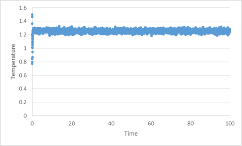
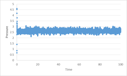
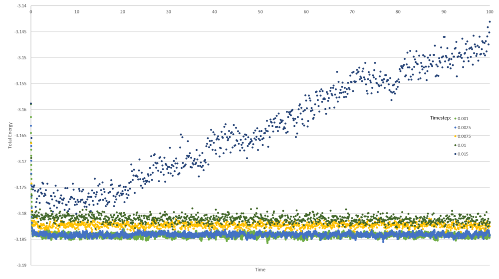
TASK: make plots of the energy, temperature, and pressure, against time for the 0.001 timestep experiment (attach a picture to your report). Does the simulation reach equilibrium? How long does this take? When you have done this, make a single plot which shows the energy versus time for all of the timesteps (again, attach a picture to your report). Choosing a timestep is a balancing act: the shorter the timestep, the more accurately the results of your simulation will reflect the physical reality; short timesteps, however, mean that the same number of simulation steps cover a shorter amount of actual time, and this is very unhelpful if the process you want to study requires observation over a long time. Of the five timesteps that you used, which is the largest to give acceptable results? Which one of the five is a particularly bad choice? Why?

The graphs below illustrate how the pressure, temperature and total energy for a simulated system vary with time, which was varied with a timestep of 0.001. The values of all 3 properties can be seen to vary at the start before reaching an average value at which the property fluctuates around for the rest of the simulation. The total energy can be seen to decrease before fluctuating, which is to be expected given that a system prefers to be in its stable, lowest energy state. The pressure and temperature can be seen to increase before fluctuating, contrary to what occured for the total energy. As all properties can be seen to reach a value around which they fluctuate, it can be concluded that the system does indeed reach equilibrium, and this occurs roughly between a time of 0.3 and 0.4.

Change of energy against time	Change of temperature against time	Change of pressure against time

The plot below shows how the total energy of a simulated system varies with time for 5 different timestep values of 0.001, 0.0025, 0.0075,0.01 and 0.015.

Change of energy against time for all timesteps

It can be seen that the total energy for all timesteps reaches an equilibrium value, with the exception of a timestep value of 0.015, for which the total energy actually increases. Therefore a value of 0.0015 for timestep would be a bad choice as the simulated system does not reach equilibrium. The largest timestep value that would give acceptable results would be a value of 0.0025 as it would allow for the simulation steps to cover a large amount of actual time but still produce accurate simulation results that reflect the physical reality. Tick, correct

Running simulations under specific conditions

TASK: Choose 5 temperatures (above the critical temperature $T^{*}=1.5$), and two pressures (you can get a good idea of what a reasonable pressure is in Lennard-Jones units by looking at the average pressure of your simulations from the last section). This gives ten phase points — five temperatures at each pressure. Create 10 copies of npt.in, and modify each to run a simulation at one of your chosen $(p,T)$ points. You should be able to use the results of the previous section to choose a timestep. Submit these ten jobs to the HPC portal. While you wait for them to finish, you should read the next section.

Temperatures of 1.6,1.8, 2.0, 2.2 and 2.4 were chosen, along with pressures of 2.4 and 2.8. These pressures were chosen by looking at the change in pressure with time from the graph in the previous section, and seeing that it was around these 2 values that the pressure reached an equilibrium.

TASK: We need to choose $\gamma$ so that the temperature is correct $T=\mathfrak{𝔗}$ if we multiply every velocity $\gamma$. We can write two equations:

$E_K=\frac{3}{2}N{k}_{B}T$

$\frac{1}{2}\sum _i{m}_i{v}_i^2=\frac{3}{2}N{k}_{B}T$

Solve these to determine $\gamma$.

Multiplying all velocities by γ gives E_K in terms of the target temperature, $\mathfrak{𝔗}$:

$\frac{1}{2}\sum _i{m}_i{\gamma }^2{v}_i^2=\frac{3}{2}N{k}_B\mathfrak{𝔗}$

${\gamma }^2=\frac{\frac{3}{2}N{k}_B\mathfrak{𝔗}}{\frac{1}{2}\sum _i{m}_i{v}_i^2}$

${\gamma }^2=\frac{\frac{3}{2}N{k}_B\mathfrak{𝔗}}{\frac{3}{2}N{k}_{B}T}$

${\gamma }^2=\frac{\mathfrak{𝔗}}{T}$

$\gamma =\pm \sqrt{\frac{\mathfrak{𝔗}}{T}}$ Tick

What does this quantity represent?

TASK: Use the manual page to find out the importance of the three numbers 100 1000 100000. How often will values of the temperature, etc., be sampled for the average? How many measurements contribute to the average? Looking to the following line, how much time will you simulate?

The three numbers all relate to the calculation of average values, and their exact purposes are defined below.

100

This number specifies the timestep length between which values are to be used calculate the averages. In this case every 100 timesteps an input value will be used.

1000

Placing this number in the code specifies that LAMMPS should use this many data points to be used to calculate the averages. In this case 1000 data points are to be used.

100000

The use of this number is to stipulate how many of timesteps are to be used by LAMMPS calculate averages. In this case 100000 timesteps are to be used.

Therefore, the values of the temperature and other properties will be sampled every 100 timesteps. The number of measurements that will contribute to the average are 1000. The timestep was taken to be 0.0025, so if 100000 timesteps were used to calculate the averages, the amount of time that will be simulated is given by 100000 x 0.025 = 250. Tick

TASK: When your simulations have finished, download the log files as before. At the end of the log file, LAMMPS will output the values and errors for the pressure, temperature, and density $\left(\frac{N}{V}\right)$. Use software of your choice to plot the density as a function of temperature for both of the pressures that you simulated. Your graph(s) should include error bars in both the x and y directions. You should also include a line corresponding to the density predicted by the ideal gas law at that pressure. Is your simulated density lower or higher? Justify this. Does the discrepancy increase or decrease with pressure?

Change of density with temperature at a pressure of 2.4	Change of density with temperature at a pressure of 2.8

The plots above shows how the density changes with temperature at 2 different pressures of 2.4 and 2.8. Both graphs show that as the temperature increases, the density decreases linearly, which corresponds to the system expanding. The predicted densities by the ideal gas law are also displayed on the graphs. By comparing the predicted and calculated densities, it can be seen that the calculated densities for both pressures are lower than that predicted by the ideal gas law. This is mainly due to one of the assumptions made by the ideal gas law. The ideal gas law assumes that there are no interactions between any of the particles in a system, which means that the density is not affected by attractive or repulsive forces.Therefore, particles can be close proximity to each other and there will be no change in the potential experienced by each particle, leading to a higher density being predicted by the ideal gas law. As the simulation uses a Lennard-Jones potential which takes into account the attractive and repulsive forces, the calculated values for density do take into account the interactions between particles, better accurately describing the system. This balance of attractive and repulsive forces leads to a lower density being obtained from the simulation. Additionally, it can be seen that this discrepancy does not change with a change in pressure. Nice explanation

Calculating heat capacities using statistical physics

TASK: As in the last section, you need to run simulations at ten phase points. In this section, we will be in density-temperature $({\rho }^{*},T^{*})$ phase space, rather than pressure-temperature phase space. The two densities required at $0.2$ and $0.8$, and the temperature range is $2.0,2.2,2.4,2.6,2.8$. Plot $C_V/V$ as a function of temperature, where $V$ is the volume of the simulation cell, for both of your densities (on the same graph). Is the trend the one you would expect? Attach an example of one of your input scripts to your report.

The graph below shows how the heat capacity divided by volume changes with increasing temperatures at 2 different densities of 0.2 and 0.8.

Change of Cv/V against temperature

For both densities, the general trend of the heat capacity of the system decreasing as the temperature increasing can be seen. This can be rationalised by considering the change in the population of the energy levels of the system with temperature. As temperature increases, higher energy states become populated, and once all the levels are populated evenly, there is little change in entropy for small changes in temperature and thus a lower specific heat capacity. Tick, nice. How is this represented energetically?

The expected trend is given by the equipartition theorem which gives the result that the heat capacity should be equal to 3R/2(where R is the gas constant), i.e. the heat capacity should be a constant. The plots clearly show that the heat capacity for both densities are not a constant, which is a result of the finite energy levels.

Increasing the density of the system from 0.2 to 0.8 can be seen to lead to a increase in the value of the heat capacity. As the volume of the system is held constant, increasing density is equal to an increase in mass, which means for any given volume, there are more atoms in the system at a higher density which would require more energy to change the temperature. Tick

The script used to calculate the heat capacity at a density of 0.8 is shown below.

### DEFINE DENSITY ###
variable d equal 0.8


### DEFINE SIMULATION BOX GEOMETRY ###
lattice sc ${d}
region box block 0 15 0 15 0 15
create_box 1 box
create_atoms 1 box

### DEFINE PHYSICAL PROPERTIES OF ATOMS ###
mass 1 1.0
pair_style lj/cut/opt 3.0
pair_coeff 1 1 1.0 1.0
neighbor 2.0 bin

### SPECIFY THE REQUIRED THERMODYNAMIC STATE ###
variable T equal 2.0 
variable timestep equal 0.0025 

### ASSIGN ATOMIC VELOCITIES ###
velocity all create ${T} 12345 dist gaussian rot yes mom yes

### SPECIFY ENSEMBLE ###
timestep ${timestep}
fix nve all nve 

### THERMODYNAMIC OUTPUT CONTROL ###
thermo_style custom time etotal temp press
thermo 10

### RECORD TRAJECTORY ###
dump traj all custom 1000 output-1 id x y z

### SPECIFY TIMESTEP ###

### RUN SIMULATION TO MELT CRYSTAL ###
run 10000
unfix nve
reset_timestep 0

### BRING SYSTEM TO REQUIRED STATE ###
variable tdamp equal ${timestep}*100
fix nvt all nvt temp ${T} ${T} ${tdamp} 
run 10000
unfix nvt
fix nve all nve 
reset_timestep 0

### MEASURE SYSTEM STATE ###
thermo_style custom step etotal temp atoms vol
variable energy equal etotal
variable energy2 equal etotal*etotal
variable temp equal temp
variable temp2 equal temp*temp
variable w equal atoms
variable x equal atoms*atoms
variable vol equal vol
fix aves all ave/time 100 1000 100000 v_energy v_energy2  v_temp v_temp2  
run 100000

variable aveetotal equal f_aves[1]
variable aveetotal2 equal f_aves[2]
variable avetemp equal f_aves[3]
variable aveetotal3 equal f_aves[1]*f_aves[1]
variable cv equal ${x}*(${aveetotal2}-${aveetotal3})/(${avetemp}*${avetemp}) 
variable cvv equal (${x}*(${aveetotal2}-${aveetotal3})/(${avetemp}*${avetemp}))/vol




print "Results"
print "--------"
print "Temperature: ${avetemp}"
print "Density: ${d}"
print "Cv: ${cv}"
print "Cv/V : ${cvv}"

Structural properties and the radial distribution function

TASK: perform simulations of the Lennard-Jones system in the three phases. When each is complete, download the trajectory and calculate $g(r)$ and $\int g(r)\mathrm{d}r$. Plot the RDFs for the three systems on the same axes, and attach a copy to your report. Discuss qualitatively the differences between the three RDFs, and what this tells you about the structure of the system in each phase. In the solid case, illustrate which lattice sites the first three peaks correspond to. What is the lattice spacing? What is the coordination number for each of the first three peaks?

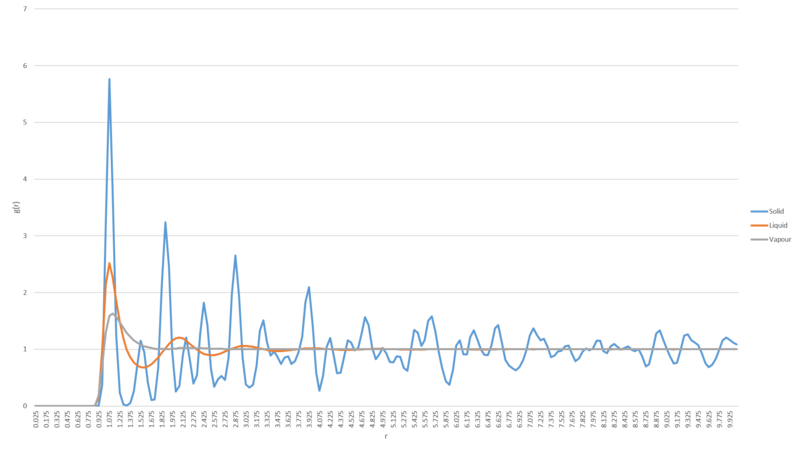
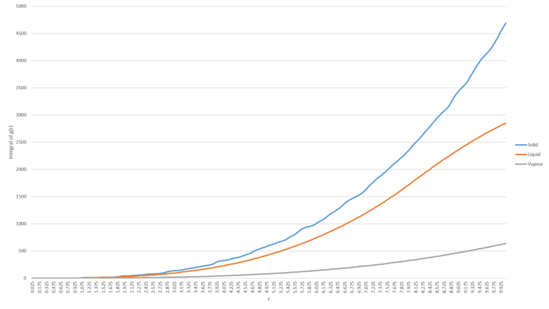
The figure on the left below shows how the Radial Distribution Function(RDF), g(r), for a system varies as the distance,r, from a reference atom in the system increases. The figure on the right meanwhile, shows how the integral of g(r) for a system varies as the value of r increases.

Change of the radial distribution function against distance for the solid, liquid and vapour phases	Integral of the radial distribution function against distance for the solid, liquid and vapour phases

The RDF is a measure of how much electron density is found at a given value of r, and allows us to study the type of order present in a system. By looking at how the RDF varies with distance for the three phases, we can see a number of features that distinguish the calculated function for each phase from each other. The RDF for the solid shows a large number of well-defined peaks with large amplitudes. This relates to the ordered nature of atoms in a solid with the peaks corresponding to the electron density of the neighbouring atoms, and the large amplitude of peaks being given by the high density of a solid. The RDF for the liquid displays how they have some degree of order, with the presence of less peaks than the RDF of the solid, which were also more defined than the peaks for the liquid. Finally, the RDF for the vapour phase highlights the highly disordered nature of the system, shown by the presence of one maxima before rapidly decreasing to a value of 1, showing there is very little medium and long range order. Tick

There are also general features that are displayed by all the RDFs for all phases. Below distances of around 1, the RDFs all go to 0, which is to be expected given that below this distances, the atoms would have to be overlapping. As the distance from the reference atom increases, the RDF for all phases approaches a value of 1. However, the RDF for the solid can be seen to fluctuate around 1, whereas the RDFs for the liquid and vapour are almost linear at 1, which further highlights the greater degree of medium and long range order in the solid. Furthermore, the rdf for solid is not that smooth - why? (dynamic averaging)

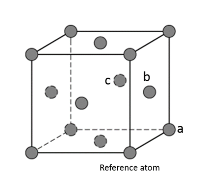
The figure below shows an illustration of the lattice sites to which the first three peaks of the RDF of the solid correspond to.

Lattice sites corresponding to the first 3 maxima peaks

The first three maxima peaks from the solid phase RDF are (1.075,5.768), (1.525,1.150), and (1.875,3.242). The lattice spacing is equal to the distance between the reference atom and atom a shown in the diagram above, which corresponds to the second peak in the radial distribution function, which gives a lattice spacing of 1.525.

The coordination number for the first three peaks at distances of 1.025, 1.525 and 1.875 are 12,6, and 24 respectively. Tick

Dynamical properties and the diffusion coefficient

TASK: In the D subfolder, there is a file liq.in that will run a simulation at specified density and temperature to calculate the mean squared displacement and velocity auto correlation function of your system. Run one of these simulations for a vapour, liquid, and solid. You have also been given some simulated data from much larger systems (approximately one million atoms). You will need these files later.

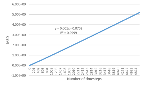
TASK: make a plot for each of your simulations (solid, liquid, and gas), showing the mean squared displacement (the "total" MSD) as a function of timestep. Are these as you would expect? Estimate $D$ in each case. Be careful with the units! Repeat this procedure for the MSD data that you were given from the one million atom simulations.

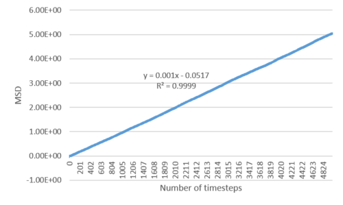
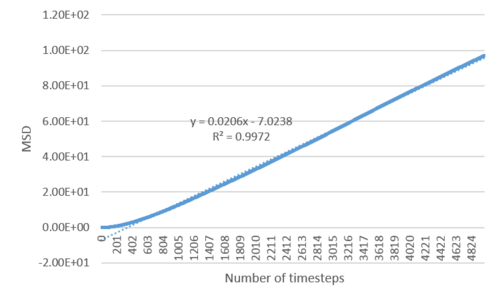
The graphs below show the how the MSD changes with time for a solid, liquid and gas, for 2 systems, one that is small, and the other that consists of 1 million atoms.

	Phase
	Solid	Liquid	Gas
MSD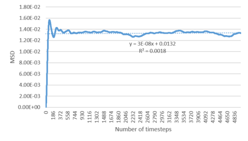
MSD (1 million atoms)

The table below summarises the diffusion coefficient calculated using the MSD from the curves above, using the following formula to calculate the coefficient $D=\frac{1}{6}\frac{\partial ⟨r^2\left(t\right)⟩}{\partial t}$

where the gradient of the MSD curves gave the value of $r^2(t)$, and where $\partial t$ was equal to the timestep of 0.002 that was used in the simulation.

	Diffusion coefficient
	MSD	MSD (1 million atoms)
Solid	2.500x10-6	4.167x10-6
Liquid	0.0833	0.0833
Gas	1.717	2.542

The trend that can be seen in the graphs and calculated values of the diffusion coefficient match up to what would be expected in real life, namely that from solid to liquid to gas, the value of D increases. This is to be expected given that the number of degrees of freedom is greater for a gas, then a liquid, and then a solid. This is due to the highly ordered nature of a solid, which restricts the ability of atoms or molecules to move around, leading to low diffusion and hence a low diffusion coefficient. Liquids are not as regularly ordered, and so has a greater degree of freedom leading to better diffusion and a higher value of D. It should be noted how increasing the size of the liquid system to 1 million atoms did not result in a change in the calculated diffusion coefficient. A gas meanwhile, has almost no order due to its constituent atoms not being fixed in space, leading to the greatest number of degrees of freedoms for all phases and a higher diffusion coefficient due to the ease of movement. Tick

For both the simulations with 1 million atoms and the simulation for a smaller scale system, the MSD for the solid phase shows the behaviour of increasing rapidly to a maxima at around 185 timesteps, then fluctuating around an average value as the timestep increased. The shape and value of the MSD for the solid differed for the different size systems, with the 1 million atoms simulations giving a graph with greater values for the MSD, along with a curve that did not fluctuate as greatly at large numbers of timesteps, which occurred in the smaller scale system. In the case of the liquid phase, both size systems showed a linear relationship between the MSD and number of timesteps. For both size systems in the gas phase, the MSD shows an exponential like behaviour with timestep at a low number of timesteps, before showing a linear relationship at a high number of timesteps. The MSD curve for 1 million atoms in the gas phase slightly differs from the smaller scale system, with a greater degree of exponential like behaviour. Tick

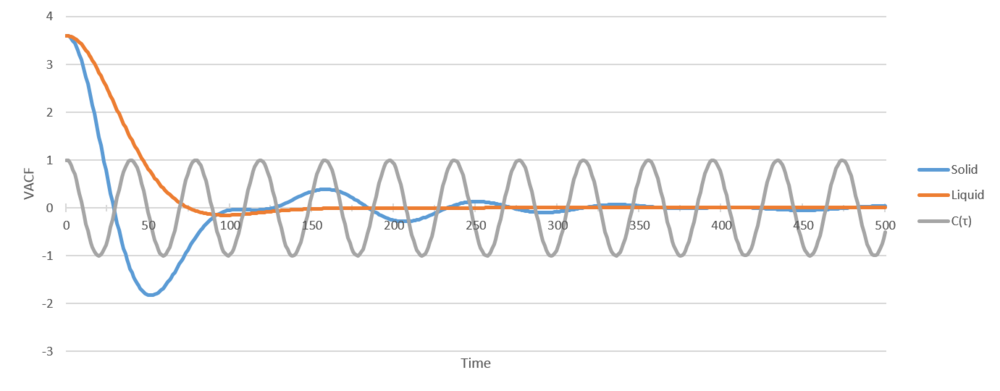
TASK: In the theoretical section at the beginning, the equation for the evolution of the position of a 1D harmonic oscillator as a function of time was given. Using this, evaluate the normalised velocity auto correlation function for a 1D harmonic oscillator (it is analytic!):

$C\left(\tau \right)=\frac{\underset{-\mathrm{\infty }}{\overset{\mathrm{\infty }}{\int }}v\left(t\right)v(t+\tau )\mathrm{d}t}{\underset{-\mathrm{\infty }}{\overset{\mathrm{\infty }}{\int }}{v}^2\left(t\right)\mathrm{d}t}$

To calculate $C\left(\tau \right)$, an equation for $v\left(t\right)$ must be known, and can be determined using $x\left(t\right)$

The equation for the evolution of the position of a 1D harmonic oscillator as a function of time is: $x\left(t\right)=A\cos (\omega t+\varphi )$

The velocity for a 1D harmonic oscillator can then be defined as: $v\left(t\right)=\frac{\partial x(t)}{\partial t}=-\omega A\sin (\omega t+\varphi )$

$C\left(\tau \right)=\frac{\underset{-\mathrm{\infty }}{\overset{\mathrm{\infty }}{\int }}v\left(t\right)v(t+\tau )\mathrm{d}t}{\underset{-\mathrm{\infty }}{\overset{\mathrm{\infty }}{\int }}{v}^2\left(t\right)\mathrm{d}t}$

$=\frac{\underset{-\mathrm{\infty }}{\overset{\mathrm{\infty }}{\int }}(-\omega A\sin (\omega t+\varphi ))(-\omega A\sin (\omega (t+\tau )+\varphi ))\mathrm{d}t}{\underset{-\mathrm{\infty }}{\overset{\mathrm{\infty }}{\int }}(-\omega A\sin (\omega t+\varphi ){)}^2\mathrm{d}t}$

$=\frac{\underset{-\mathrm{\infty }}{\overset{\mathrm{\infty }}{\int }}(-\omega A\sin (\omega t+\varphi ))(-\omega A\sin (\omega t+\omega \tau +\varphi ))\mathrm{d}t}{\underset{-\mathrm{\infty }}{\overset{\mathrm{\infty }}{\int }}(-\omega A\sin (\omega t+\varphi ){)}^2\mathrm{d}t}$

$=\frac{\underset{-\mathrm{\infty }}{\overset{\mathrm{\infty }}{\int }}(\omega A\sin (\omega t+\varphi ))(\omega A\sin (\omega t+\omega \tau +\varphi ))\mathrm{d}t}{\underset{-\mathrm{\infty }}{\overset{\mathrm{\infty }}{\int }}{\omega }^2{A}^2{\sin }^2(\omega t+\varphi )\mathrm{d}t}$

$=\frac{\underset{-\mathrm{\infty }}{\overset{\mathrm{\infty }}{\int }}(\omega A\sin (\omega t+\varphi ))(\omega A(\sin (\omega t+\varphi )\cos (\omega t)+\cos (\omega t+\varphi )\sin (\omega t)))\mathrm{d}t}{\underset{-\mathrm{\infty }}{\overset{\mathrm{\infty }}{\int }}{\omega }^2{A}^2{\sin }^2(\omega t+\varphi )\mathrm{d}t}$

$=\frac{{\omega }^2{A}^{2}cos(\omega t)\underset{-\mathrm{\infty }}{\overset{\mathrm{\infty }}{\int }}(si{n}^2(\omega t+\varphi ))}{{\omega }^2{A}^2\underset{-\mathrm{\infty }}{\overset{\mathrm{\infty }}{\int }}(si{n}^2(\omega t+\varphi ))dt}+\frac{{\omega }^2{A}^{2}sin(\omega t)\underset{-\mathrm{\infty }}{\overset{\mathrm{\infty }}{\int }}(sin(\omega t+\varphi )cos(\omega t+\varphi ))}{{\omega }^2{A}^2\underset{-\mathrm{\infty }}{\overset{\mathrm{\infty }}{\int }}(si{n}^2(\omega t+\varphi ))dt}$

$=cos(\omega t)+\frac{sin(\omega t)\underset{-\mathrm{\infty }}{\overset{\mathrm{\infty }}{\int }}(sin(\omega t+\varphi )cos(\omega t+\varphi ))}{\underset{-\mathrm{\infty }}{\overset{\mathrm{\infty }}{\int }}(si{n}^2(\omega t+\varphi ))dt}$

$=cos(\omega t)$ Good

Change of the VACF against time for solid and liquid phases compared to the harmonic oscillator

The graph above shows how the VACF changes with time for a solid phase, liquid phase, and for the harmonic oscillator. The VACF for the harmonic oscillator shows an oscillating relationship around 0 that can be represented using a cos curve. The long range order in a solid can be seen in the obtained curve, with the VACF slowly decreasing while fluctuating around 0 as time increases, before the fluctuations become negligible and a straight line can be observed. The curve for liquid highlights how there is less long range order in a liquid than in a solid, as the curve hardly fluctuates around 0, and instead decreases to a slight minima around a time of 100, before showing a straight line for the remainder of the simulation. Comparison of the curves for both phases to the harmonic oscillator curve highlights how the phases can not be accurately represented by a harmonic oscillator. Tick but could discuss in more detail

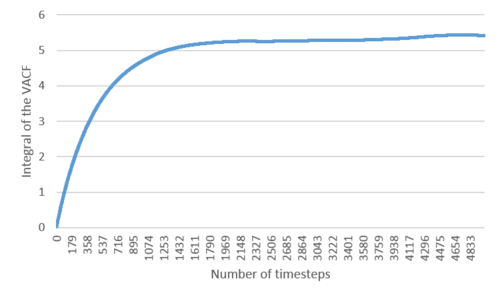
TASK: Use the trapezium rule to approximate the integral under the velocity auto correlation function for the solid, liquid, and gas, and use these values to estimate $D$ in each case. You should make a plot of the running integral in each case. Are they as you expect? Repeat this procedure for the VACF data that you were given from the one million atom simulations. What do you think is the largest source of error in your estimates of D from the VACF?

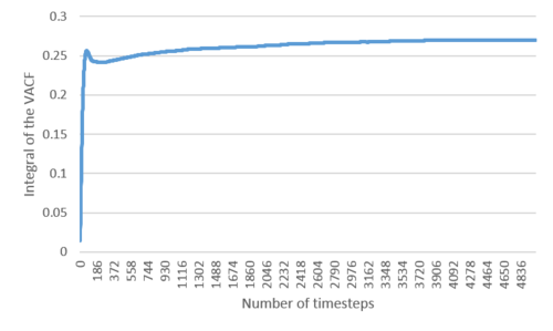
The graphs below show the how the integral of the VACF changes with time for a solid, liquid and gas. As for the MSD calculations, a small size system and a system of 1 million atoms were studied.

	Phase
	Solid	Liquid	Gas
Integral of the VACF
Integral of the VACF (1 million atoms)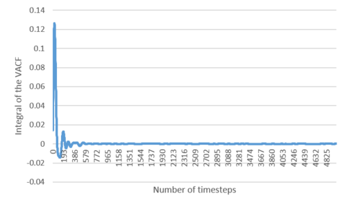

The table below summarises the diffusion coefficient calculated using the integral of the VACF from the curves above, using the following formula to calculate the coefficient $D=\frac{1}{3}\underset{0}{\overset{\mathrm{\infty }}{\int }}\mathrm{d}\tau ⟨\mathbf{v}\left(0\right)\cdot \mathbf{v}\left(\tau \right)⟩$

	Diffusion coefficient
	VACF	VACF (1 million atoms)
Solid	8.00962x10-5	4.55295x10-5
Liquid	0.097888878	0.090091476
Gas	1.808192418	3.268465798

A similar trend that can be seen in the calculated values of the diffusion coefficient calculated using the integral of the VACF to the coefficients calculated using the MSD, shown by an increase in the value of D as the phase changes from solid to liquid to gas. This comes as no surprise due to the fact that we are simply calculating the values using a different method rather than changing any parameters of the simulation. As for the coefficients calculated using the MSD, the value of D calculated using the integral of the VACF for the liquid phase shows the least difference when moving from a small scale system to 1 million atoms. Tick

It can be seen that for all phases, the plots of the integral of the VACF are highly different from the MSD plots obtained. For both size systems, the integral for the solid phase shows the behaviour of increasing rapidly to a maxima at around 50 timesteps, then rapidly decreasing to a negative integral before fluctuating around an integral value of 0 as the timestep increased. For 1 million atoms in the solid phase, the integral took less timesteps to reach 0, while also obtaining higher value integrals than for the smaller scale system. For the liquid phase, the integrals for both size systems increased rapidly to a maximum, dropped slightly and the very slowly increased with the number of timesteps. The curve for 1 million atoms is much smoother than the curve for a smaller scale liquid system, but still gave integrals of a similar value. For the gas phase, both size systems showed a logarithmic type relationship, with the curve for 1 million atoms showing a more gradual change in the integral than the curve for the small scale system, which increased and leveled off rapidly. The obtained integral values for the 1 million atoms simulation were also larger than those obtained for the smaller scale system.

The largest source of error in the estimated value of the diffusion coefficient from the VACF arises from the use of the trapezium rule to calculate the area under the curve. As the rule works by splitting the area under a curve into a number of trapeziums, it is possible for this area to be over or underestimated depending on the nature of the curve, and this error is a cumulative process due to the use of a sum to calculate the total area under the curve. This error could be reduced by using more trapeziums of smaller width to estimate the integral, but as the width of the trapezium is equal to the timestep used in the simulation, this would require a larger amount of computational cost. Tick, any other sources of error?

Comparison of the diffusion coefficients calculated using the MSD and VACF integral shows us that there is a great deal of similarity between the two, with the obtained values of D being on the same order of magnitude for all phases for both size systems. Any possible difference in the values given between the two methods could come from the way in which they were calculated, with the gradient of the curve being used for the MSD method, and the integral of the curve being used for the VACF method. Tick

Conclusion

In this laboratory, simulations were used to study a simple liquid and calculate its structural and dynamic properties, such as the Radial Distribution Function and heat capacity. Through the use of the velocity-Verlet algorithm, it was shown that the use of numerical integration to solve the differential equations that describe properties of a system can introduce errors, which stem from the choice of timesteps used in a simulation.

The timestep chosen for a simulation was found to have an effect on whether a simulated system attained a state of equilibrium. For the study of how total energy varies with time for a system, a larger timestep resulted in the system not attaining a equilibrium state, whereas all other timesteps used showed the expected result of fluctuations of the total energy of the system around an average value. Density as a function of temperature was plotted for 5 temperatures at 2 different pressures, and then compared to the density predicted by the ideal gas law. The ideal gas law was found to give density values higher than those found by the simulation, and can be interacted to the law not taking into account interactions between the particles being studied.

The variation of heat capacity with temperature was then studied, and was found to decrease as temperature increased, which is the opposite of what is expected ideally. This is thought to be down to the system reaching a point where it can longer absorb any more energy.The Radial Distribution Function and its integral were used to characterise the structure for the solid, liquid, and vapour phases of a Lennard-Jones fluid.The shape of the function was shown to be powerful in distinguishing the phases due to the function for each phase showing a different number of peaks which had different amplitudes.

Finally, the mean squared displacement and velocity auto correlation function of a system was measured. These were then used to calculate the diffusion coefficient for solid, liquid and vapour phases, which were found to follow the expected trend. Comparison of the obtained coefficients from the MSD and VACF showed an agreement between the two methods, with only a slight difference between the two being observed.