Talk:Mod:lt912 ising
Ising Model Computational Experiment
Introduction to the Ising Model
The Model
In the presence of no external magnetic fields, the energy of the model is given by:
where is the total interaction energy between spins in adjacent lattice cells and is a constant determining the strength of the interaction. The term is the spin of a particular cell.
Energy is minimized in the model when all the spins are aligned in the same direction, either up or down. Two adjacent spins can combine in the following ways:
Due to the negative term in the interaction energy equation, the minimum energy occurs when the product is maximized - either or . The total energy then depends on the number of interactions available in the lattice. This depends on both the number of cells , and the dimensionality of the lattice . Due to periodic boundary conditions any edge cells have the same number of interactions as all others.
Starting with the 1 dimensional case it can easily be seen that each cell is adjacent to 2 others, hence the total number of interactions is . When the lattice is extended to another dimension each cell has 2 interactions on the new axis as well. Therefore in the 2D case the interaction number is and using the same logic the 3D case is . The general case is therefore . Substituting this into the total energy equation to find the minimum energy of a lattice:
The multiplicity of the minimum energy state is 2 as it can be reached with all the spins pointing either up or down. Entropy can be calculated using where therefore .
NJ: good explanation, but include the numerical value of the entropy too.
Phase Transitions
TASK: Imagine that the system is in the lowest energy configuration. To move to a different state, one of the spins must spontaneously change direction ("flip"). What is the change in energy if this happens ()? How much entropy does the system gain by doing so?
The minimum energy value in this case is . When the spin of one cell in the lowest energy state is flipped, the new state loses replaces some stabilizing interactions with destabilizing ones. The energy value of this system is given by . Where the one positive energy term represents the loss of the stabilizing interaction when a spin is flipped and the other is the addition of new destabilizing interactions. Therefore in this system the energy when one spin is anti parallel is and the energy change is .
The number of states of a system of N particles where 1 spin is flipped 2N. This is because each energy state still has a multiplicity of 2, as (N-1) spins up and 1 spins is equivalent to (N-1) spins down and 1 spin up. Furthermore the N is present as any of of the N spins can flip. Therefore:
TASK: Calculate the magnetisation of the 1D and 2D lattices in figure 1. What magnetisation would you expect to observe for an Ising lattice with at absolute zero?
The 1D and 2D cases both have a total magnetization of +1. A 3D lattice of 1000 cells at absolute 0 would likely have a total magnetization of either +1000 or -1000.
NJ: excellent!
Calculating the Energy and Magnetization
Modifying the Files
TASK: complete the functions energy() and magnetisation(), which should return the energy of the lattice and the total magnetisation, respectively. In the energy() function you may assume that at all times (in fact, we are working in reduced units in which , but there will be more information about this in later sections). Do not worry about the efficiency of the code at the moment — we will address the speed in a later part of the experiment.
File emailed holding relevant code: IsingLattice - Before Acceleration - Lukas Turcani.py
The energy is calculated by . However this notation describes a process which goes through every cell in the lattice, calculates its interaction with the other cells (the product of their spins) and returns a sum of these interactions. This means every interaction is counted twice as the interaction is the same as . This means that the factor of has to be introduced.
The code written for this task still cycles through every cell, however only a cell's interaction with the ones 1 row or column in front is summed. This means every interaction is considered but a factor of is unnecessary. Due to periodic boundary conditions, the first column is treated as in front of the last one, similarly the first row is in front of the last.
The magnetization was calculated through the series . By writing a code which goes through every cell in the lattice and add its value to a running total, which is returned at the end.
def energy(self):

              "Return the total energy of the current lattice configuration."

              energy = 0.0

              #Cycle Through All Cells by selecting all indices 1 by 1

              for col in range(0, self.n_cols):

                            for row in range(0, self.n_rows):


                                          #If a Cell is in the Last Column in Interacts with Cells in the First Column


                                          if col == (self.n_cols - 1):
                                                        energy += self.lattice[col][row] * self.lattice[0][row]


                                          #Otherwise a Cell Interacts with the one in Front


                                          else:
                                                        energy += self.lattice[col][row] * self.lattice[col+1][row]


                                          #Cells in Last Row interact with Cells in First Row


                                          if row == (self.n_rows - 1):
                                                        energy += self.lattice[col][row] * self.lattice[col][0]


                                          #All Others Interact with Row in Front


                                          else:
                                                        energy += self.lattice[col][row] * self.lattice[col][row+1]


              #Energy is Negative Sum of Interactions

              energy = energy * -1
              return energy

def magnetisation(self):

              "Return the total magnetisation of the current lattice configuration."

              magnetisation = 0.0

              #Go through all the cells and add their spins

              for col in self.lattice:

                            for cell in col:
                                          magnetisation += cell
              return magnetisation
NJ: nice explanation. Well done for spotting that you only need to go "forward and down".
Testing the Files
TASK: Run the ILcheck.py script from the IPython Qt console using the command

Introduction to Monte Carlo Simulation
Average Energy and Magnetization
TASK: How many configurations are available to a system with 100 spins? To evaluate these expressions, we have to calculate the energy and magnetization for each of these configurations, then perform the sum. Let's be very, very, generous, and say that we can analyse configurations per second with our computer. How long will it take to evaluate a single value of ?
The total number of configurations is given by where is the number of possible states per particle and is the number of particles. Since each spin can be either up or down and there are 100 spins so . Therefore .
It would take years to calculate a single value of .
Modifying IsingLattice.py
TASK: Implement a single cycle of the above algorithm in the montecarlocycle(T) function. This function should return the energy of your lattice and the magnetisation at the end of the cycle. You may assume that the energy returned by your energy() function is in units of ! Complete the statistics() function. This should return the following quantities whenever it is called: , and the number of Monte Carlo steps that have elapsed.
Files emailed holding relevant code: IsingLattice - Before Acceleration - Lukas Tucani.py
The function created for implementing a single cycle of the Monte Carlo algorithm initially adds 1 to the counter of Monte Carlo steps. It then saves the energy and magnetization of the current configuration in E_0 and M_0 respectively, energy is in reduced units kB. The randomly generated numbers held in the random_i and random_j variables are used as the index of a spin in the lattice. The spin in that cell is then flipped by multiplication with -1. The energy and magnetization of the lattice after the flip is saved in E_1 and M_1. The energy change is calculated by E_1 - E_0. If the change is less than 0 the new configuration is left unchanged and its values of energy, energy squared, magnetization and magnetization squared are added to the running totals. If the energy change is greater or equal to 0 a randomly generated number between 0 and 1 is compared to . If the number is less than or equal to this, the new configuration is left unchanged and its values of energy, energy squared, magnetization and magnetization squared are added to the running totals. However if the number is greater than this the cell is flipped back by another multiplication with -1.
The statistics function takes the running totals of energy, energy squared, magnetization and magnetization squared and divides them by the running total of Monte Cycles performed.
NJ: Much quicker to use np.exp(X) than np.e ** X, but the algorithm is all correct.
def montecarlostep(self, T):

              # complete this function so that it performs a single Monte Carlo step

              #the following two lines will select the coordinates of the random spin for you

              random_i = np.random.choice(range(0, self.n_rows))

              random_j = np.random.choice(range(0, self.n_cols))

              #the following line will choose a random number in the range [0,1) for you

              random_number = np.random.random()

              #Add 1 to cycle counter

              self.n_cycles += 1.0

              #Create variables for energy (reduced, kB units) and magnetisation of configuration before MC step

              E_0 = self.energy()

              M_0 = self.magnetisation()

              #Take MC step

              self.lattice[random_j][random_i] = -1 * self.lattice[random_j][random_i]

              #Create variables for energy and magnetisation of configuration after MC step

              E_1 = self.energy()

              M_1 = self.magnetisation()

              #Calculate change in energy across MC step

              E_change = E_1 - E_0

              #If energy change is <0 accept the new configuration

              if E_change < 0:

                            E_0 = E_1
                            M_0 = M_1
                            self.E += E_0
                            self.M += M_0
                            self.E2 += (E_0**2)
                            self.M2 += (M_0 **2)
              if E_change >= 0:

                            #If energy change is >0 AND random number generated is < or = likelyhood of step - accept the new configuration

                            if random_number <= np.e ** (-1 * E_change / T):
                                          E_0 = E_1
                                          M_0 = M_1
                                          self.E += E_0
                                          self.M += M_0
                                          self.E2 += (E_0 ** 2)
                                          self.M2 += (M_0 **2)
                            #If energy change is >0 AND random number generated is > likelyhood of step - reject the new configuration (ie revert to old one)

                            if random_number > np.e ** (-1 * E_change / T):


                                          self.E += E_0

                                          self.M += M_0
                                          self.E2 += (E_0 ** 2)
                                          self.M2 += (M_0 ** 2)
                                          self.lattice[random_j][random_i] = -1 * self.lattice[random_j][random_i]
                                          # the function should end by calculating and returning both the energy and magnetisation:

              return self.energy(), self.magnetisation()

def statistics(self):

              # complete this function so that it calculates the correct values for the averages of E, E*E (E2), M, M*M (M2), and returns them

              aveE = self.E / self.n_cycles

              aveE2 = self.E2 / self.n_cycles

              aveM = self.M / self.n_cycles

              aveM2 = self.M2 / self.n_cycles

              return aveE, aveE2, aveM, aveM2, n_cycles
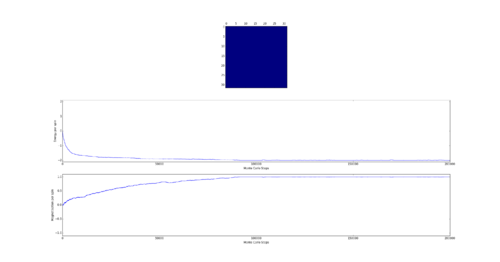
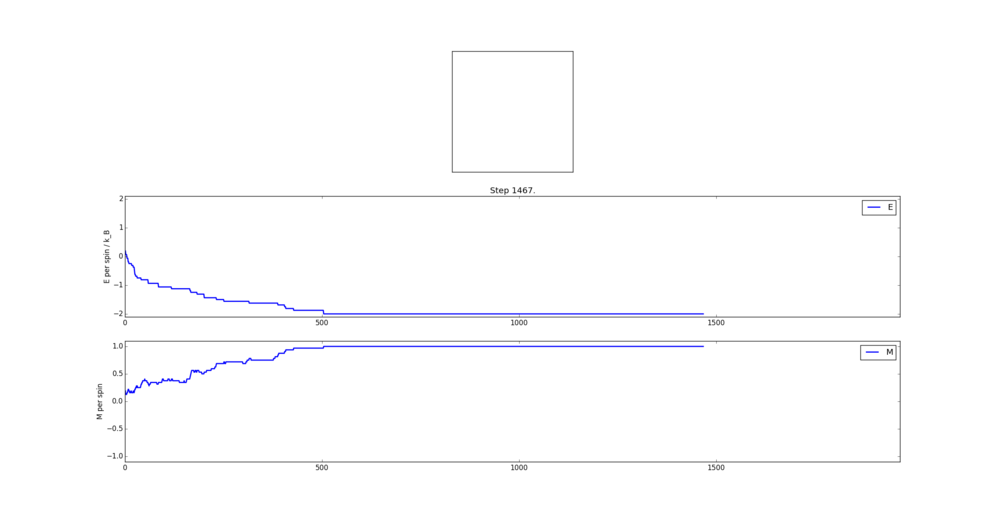
TASK: If , do you expect a spontaneous magnetisation (i.e. do you expect )? When the state of the simulation appears to stop changing (when you have reached an equilibrium state), use the controls to export the output to PNG and attach this to your report. You should also include the output from your statistics() function.
Curie Temperature is the point below which spins spontaneously align. Therefore below the Curie temperature spontaneous magnetization is expected. This can be either complete such as at absolute 0 or partial such as in iron ferromagnets at room temperature which have magnetic domains of similarly aligned spins.
The output of the statistics function:
Averaged quantities: ('E = ', -1.7980416666666668) ('E*E = ', 3.4063098958333335) ('M = ', 0.8926458333333334) ('M*M = ', 0.8500462239583333)
Accelerating the Code
TASK: Use the script ILtimetrial.py to record how long your current version of IsingLattice.py takes to perform 2000 Monte Carlo steps. This will vary, depending on what else the computer happens to be doing, so perform repeats and report the error in your average!
The standard error was found with the following equation:
where:
| Run Number | Time Taken / seconds |
|---|---|
| 1 | 8.43443997951 |
| 2 | 9.6322162045 |
| 3 | 9.16701344299 |
| 4 | 9.30342627048 |
| 5 | 9.34671405487 |
| 6 | 8.63034164173 |
| 7 | 8.61251769462 |
| 8 | 8.44312635686 |
| 9 | 8.98462825688 |
| 10 | 8.33761712938 |
| Average | 8.889204
STD Error: 0.136852 |
TASK: Look at the documentation for the NumPy sum function. You should be able to modify your magnetisation() function so that it uses this to evaluate M. The energy is a little trickier. Familiarise yourself with the NumPy roll and multiply functions, and use these to replace your energy double loop (you will need to call roll and multiply twice!).
File emailed holding relevant code: IsingLattice - After Acceleration - Lukas Turcani.py
The magnetisation function simply requries numpy's sum function applied to the lattice. This sums the value of every cell.
It was previously mentioned that the energy is calculated by taking the product of a cell with the ones in the column and row in front of it and then summing all of the products. The use of roll and multiply functions allows the creation of 2 matrices which together hold all of these products. The combined total of summing these matrices as in the magnetisation case produces the negative energy.
The method is this:
The roll function first shifts the lattice so that each cell moves to the column in front (periodic boundary conditions apply), forming a new lattice L1. L1 is multiplied by the original lattice, L0, with the multiply function. This forms a third lattice L2. Each cell in L2 holds the product of the cells in L0 and L1 with the same index. Sum all the cells in L2. This is the same as taking the product of every cell with the one in the column in front and summing all the products.
Repeat but shift row-wise.
Combine the two sums to give the negative energy.
Multiply by negative one to find the total energy.
The code is:
def energy(self):

              "Return the total energy of the current lattice configuration."

              #Form a new lattice where each cell occupies the column in front


              lattice_roll_col = np.roll(self.lattice,1,axis=1)

              #Form a new lattice where each cell occupies the row in front

              lattice_roll_row = np.roll(self.lattice,1,axis=0)

              #Multiply the translated lattices with the original. Take the negative sum of the resulting lattices.

              energy = -1 * np.sum(np.multiply(self.lattice,lattice_roll_col) + np.multiply(self.lattice, lattice_roll_row))

              return energy

def magnetisation(self):

              "Return the total magnetisation of the current lattice configuration."


              #Go through all the cells and add their spins


              magnetisation = np.sum(self.lattice)

              return magnetisation
TASK: Use the script ILtimetrial.py to record how long your new version of IsingLattice.py takes to perform 2000 Monte Carlo steps. This will vary, depending on what else the computer happens to be doing, so perform repeats and report the error in your average!
| Run Number | Time Taken / seconds |
|---|---|
| 1 | 0.427938 |
| 2 | 0.275911 |
| 3 | 0.273554 |
| 4 | 0.274325 |
| 5 | 0.268116 |
| 6 | 0.264556 |
| 7 | 0.272125 |
| 8 | 0.276326 |
| 9 | 0.266286 |
| 10 | 0.280874 |
| Average | 0.288001
STD Error:0.014826 |
NJ: Very good. Sometimes doing things the non-intuitive way is much quicker!
The Effect of Temperature
Correct the Average Code
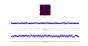
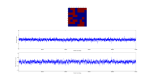
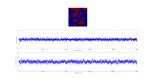
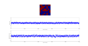
TASK: The script ILfinalframe.py runs for a given number of cycles at a given temperature, then plots a depiction of the final lattice state as well as graphs of the energy and magnetisation as a function of cycle number. This is much quicker than animating every frame! Experiment with different temperature and lattice sizes. How many cycles are typically needed for the system to go from its random starting position to the equilibrium state? Modify your statistics() and montecarlostep() functions so that the first N cycles of the simulation are ignored when calculating the averages. You should state in your report what period you chose to ignore, and include graphs from ILfinalframe.py to illustrate your motivation in choosing this figure.
Files emailed holding relevant code: ILfinalframe_lukas_turcani.py + probability_distribution_plotter_lukas_turcani.py + convergence_vs_lattice_size_lukas_turcani.py + IsingLattice - After Acceleration - Lukas Turcani.py
As the Monte Carlo algorithm is stochastic, there is no guarantee that the minimum energy state will be reached within a finite number of steps. However, as the the number of allowed steps increases so does the probability that the algorithm will reach the minimum energy. To illustrate with an example, assume that for a 3x3 Ising lattice the Monte Carlo is allowed to run for 50 steps, 100 separate times. Since the initial configuration of the lattice is random, there is a small chance that the minimum energy state will be found with the first step. Likewise there is a probability that on some implementation the algorithm may not find the minimum energy state at all. Each step has its own probability of how likely the algorithm is to converge on the minimum energy on that step forming a probability distribution. If one knows the probability distribution it is possible to say that, for example, in 90% of cases the Monte Carlo algorithm will find the minimum energy state by a certain step. It is prudent then to start taking the averages after this step. The 90% figure was chosen arbitrarily - but if in 90% of cases the algorithm starts taking the average at the correct point it can be considered relatively successful. Bearing in mind that if a later step of was chosen the success rate would have been higher at the cost of longer computational time required to reach that step in every simulation. An additional point to consider is that each lattice will have its own probability distribution based on its dimensionality and number of cells.
Therefore the first step was to obtain the probability distribution of a number of lattices. This was achieved by modifying the ILfinalframe.py file to run on square lattices from 2x2 to 17x17 via a for loop. In addition, each lattice had the Monte Carlo algorithm implemented separate 1000 times. This was so that any probability distribution obtained had sufficient data to be considered valid. Since this was computationally somewhat lengthy the resulting data was written to a file so that it could be accessed quickly at a later point without needing to run all the simulations again. Each implementation was allowed to run for a maximum of 999999 steps, but was terminated the moment the minimum energy was found to save computational time. In all cases the algorithm found the minimum energy within this number of steps.
from IsingLattice import *

from matplotlib import pylab as pl

import numpy as np

from collections import Counter

#Create file that will hold list of steps at which algorithm found minimum energy step

data_file = open("data_file","w")

#run simulation on lattice sizes between 2x2 and 17x17

for lat_size in range(2,18):

              print "Lattice Size: ", lat_size

              #write the lattice size to file

              data_file.write("Lattice Size: " + str(lat_size) + "\n")

              #list which holds steps at which simulation reached minimum energy

              min_energy_step = []

              #run the simulation at this lattice size 1000 times

              for x in range(0,1000):

                            if x % 100 == 0:
                            print "Trial: ", x
                            temperature = 1.0
                            runtime= 999999
                            il = IsingLattice(lat_size, lat_size)
                            spins = float(lat_size*lat_size)
                            times = range(runtime)
                            for i in times:
                                          #perform monte carlo step

                                          energy, magnetisation = il.montecarlostep(temperature)
                                          #notify if minimum energy state was not found within 999999 MC steps

                                          if i == (runtime-1):
                                                        print "MAX NOT FOUND!!"
                                          #if minimum energy state is found record at which step it was by adding to list and move on to next simulation

                                          if energy/spins == -2:
                                                        min_energy_step.append(i)
                                                        break
              #write the list of steps at which minimum energy state was found to file

              data_file.write(str(min_energy_step) + "\n")

data_file.close()
In order to plot and analyse the data obtained another script was written to operate on the data file. The previous script generated a file which contained a list of the steps at which the Monte Carlo algorithm found the minimum energy for each lattice. This second script takes those lists and tallies how often a particular step was the step of convergence i.e. appears in the list. It then plots the data so that the step number is on the x axis and the y axis is how frequently that step was converged on. Furthermore in order to find the step by which 90% of the simulations had found the minimum energy state the script goes along the x axis, left to right, counting the number of simulations accounted for. The step at which 900 simulations are accounted for is the 90% probability of convergence step. It is also plotted on the probability distribution and saved to an additional file for further analysis.
import os as os

from matplotlib import pylab as plt

from collections import Counter

import numpy as np

os.chdir("F:\Chemistry\Year 3\Labs\Ising\ImperialChem-Year3CMPExpt-master")

#Open file holding steps on which minimum energy was reached

data_file = open("data_file", "r")

#create figure to make plots on

fig = plt.figure()

#create file to hold step on which simulations should start averaging

avging_step_file = open("avging_step_data", "w")

#go through file holding data line by line

for line in data_file:

              #split line into a list of words

              line = line.split(" ")

              xdata = []

              ydata = []

              combined_data = []

              #go through line word by word

              for x in range(0,len(line)):

                            line[x] = line[x].rstrip(",")
                            line[x] = line[x].rstrip("\n]")
                            line[x] = line[x].lstrip("[")
                            #lines longer than 3 words are made up of lists of numbers - convert these numbers to be stored as integers not strings

                            if len(line)!=3:
                                          line[x] = int(line[x])
              #lines of length 3 hold information regarding lattice size, for these lines save the lattice size info and use it to title the subplots

              if len(line) == 3:
                            curr_plot = fig.add_subplot(4,4,int(line[2])-1)
                            curr_title = curr_plot.set_title(line[2] + "x"+line[2]+" Lattice")
                            avging_step_file.write(str(line[2]))
             #lines longer than 3 words are made up of lists of numbers

             if len(line) != 3:
                            #find how often a certain step is the step at which minimum energy state is found

                            tally = Counter(line)
                            #tally is a dictionary - step number is the key, how often it appears is the value - put these into separate lists for x and y data

                            for x in tally:
                                          xdata.append(int(x))
                                          ydata.append(int(tally[x]))
                                          #list of tuples - so that each x value is coupled to its correspnding y value

                                          combined_data.append((int(x),int(tally[x])))
                            #sort data by x value

                            combined_data = sorted(combined_data)
                            total_converged = 0
                            #the step by which 900 simulations have found minimum energy step is the step by which there is 90% probability of convergence

                            for x in combined_data:
                                          total_converged += x[1]
                                          if total_converged >= 900.0:
                                                        most_converged = x[0]
                                                        break
                            #write the step by which 90% probability of convergence to file

                            avging_step_file.write(" "+str(most_converged)+"\n")
                            #plot the distribution

                            curr_plot.bar(xdata,ydata,edgecolor="b", color="b")
                            curr_axes = curr_plot.set_ylim(0,int(max(ydata)*1.5))
                            conv_line = curr_plot.axvline(x = most_converged, color = "r", linewidth = 1, label = ("90% Converged\nBy Step "+str(most_converged)))
                            curr_leg = curr_plot.legend(frameon=False)
                            curr_plot.set_xlabel("Step Number")
                            curr_plot.set_ylabel("Number of Convergences")
plt.show()

avging_step_file.close()

data_file.close()
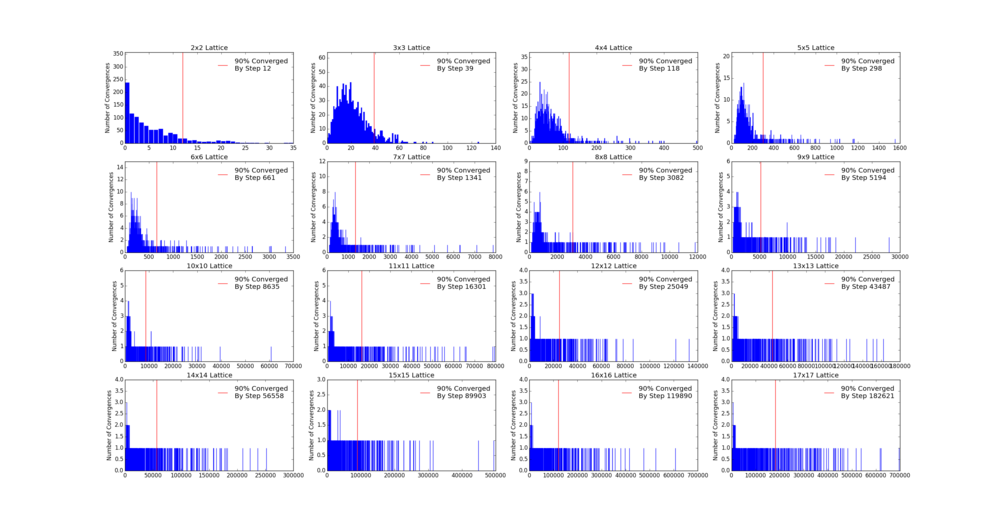
The third script reads the file containing the lattice size and number of the step by which 90% of the simulations found the minimum energy state. It then plots the number of rows or columns the lattice has against this step. From plotting this it was clear that there seems to be an exponential relationship between lattice size and the step of 90% convergence. In order to verify this the exponential function was fit to this data. The resulting fit exponential curve fit the data relatively well, with a root mean squared error of 2321. This is considering that the numbers being dealt with are 2 orders of magnitude larger than the error. This in effect provides a general formula for finding the step by which 90% of simulations will converge on the minimum energy for a square 2D lattice. The formula is:
where is the step by which 90% of simulations will converge and is the number of row or columns in the square lattice.
from matplotlib import pylab as plt

import os as os

import scipy.optimize as spo

import numpy as np

os.chdir("F:\Chemistry\Year 3\Labs\Ising\ImperialChem-Year3CMPExpt-master")

#open file containing the 90% probability of convergence step for each lattice size

data = open("avging_step_data","r")

xdata = []

ydata = []

#read file line by lie

for line in data:

              #split line into list of words and put lattice size as x data and step as y data

              line = line.split(" ")

              xdata.append(int(line[0]))

              ydata.append(int(line[1]))

#define the exponential function with 3 variables to optimize

def exp_func(x, a, b ,c):

              return (a * np.exp(b*x)) + c

#optimize the exponential function

popt , pcov = spo.curve_fit(exp_func, xdata,ydata)

#create a set of points on which to plot the exponential function

exp_xdata = np.linspace(0,18,180)

exp_ydata = []

#apply the exponential function to those points

for x in xdata:

              exp_ydata.append(exp_func(x,*popt))

#check by how much the actual step of 90% probability is different to that predicted by exponential function

diffs = np.subtract(np.asarray(ydata),np.asarray(exp_ydata))

#square the differences

diffs = np.square(diffs)

#calculate the root of the mean of the difference squared

rms = np.mean(diffs)

rms = np.sqrt(rms)

print rms

plt.plot(exp_xdata,exp_func(exp_xdata,*popt),label = "y = %d exp(%s x) %d\nRMS Error = %s" %(popt[0],str(popt[1])[0:5],popt[2],rms))

plt.scatter(xdata,ydata,marker= "x")

plt.legend()

plt.xlabel("Lattice Size ^ 0.5")

plt.ylabel("Step of 90% Convergence")

plt.show()

Next the 8x8 Lattice was tested again to see how a change in temperature effects the simulations ability to find the equilibrium state. As temperature increases, the equilibrium state will not necessarily be the minimum energy state. This makes running a for loop to run many simulations as above impractical. This is because the energy of the equilibrium state is unknown when a simulation starts and it therefore cannot be set terminate upon reaching it.
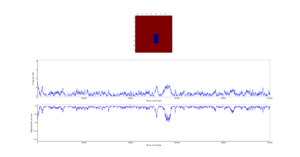
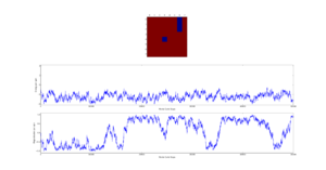
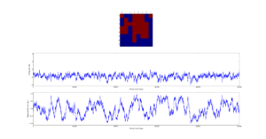
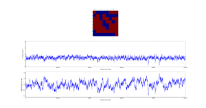
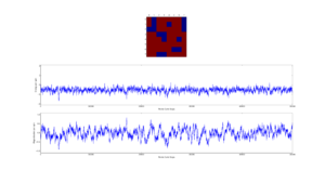
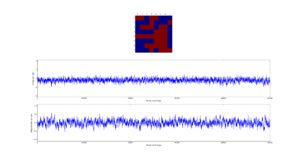
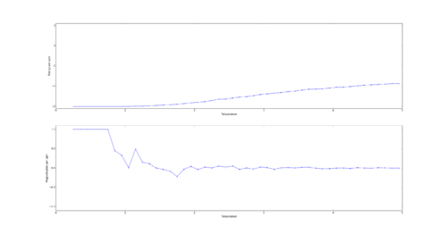
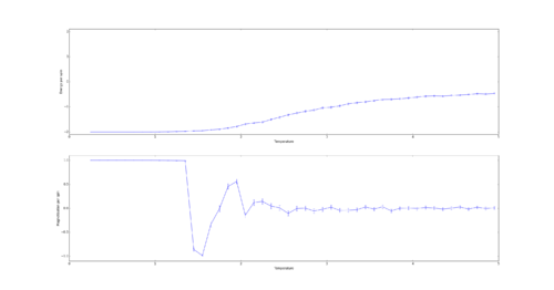
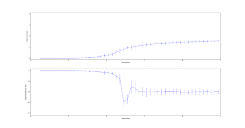
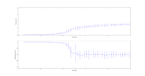
As a result the effect of temperature was examined in the following way. The 8x8 lattice was selected with temperatures in the range of 1 to 300,000. 5000 to 50,000 Monte Carlo steps were then performed, depending on the temperature. 300,000 was selected as an extreme test case to see if any unusual behavior appeared at abnormally large temperature values. The results allow the drawing of 3 conclusions. Firstly the equilibrium energy value increases from -2 per cell to 0 per cell as temperature increases. Once at 0 per cell the equilibrium energy remains at this level despite temperature increases. Secondly the number of steps required to reach the equilibrium state increases between temperature values of 1 and 1.5 and then decreases between 1.5 and 2. Above this temperature the equilibrium state is reached almost instantly. Finally, the frequency of oscillations increases as temperature increases - up to a point.
The initial increase and subsequent decrease in number of steps has to be taken with a very large grain of salt. This relies on the observations of very few attempts and as explained earlier the numbers of steps required to reach equilibrium can vary enormously - even with identical initial conditions. However, the observation that temperatures with an average equilibrium energy of 0 reach their equilibrium state almost instantly is intuitive. This because the initial configuration is random. As a result it can be considered just another random fluctuation from the average energy of 0. In other words the initial configuration falls within the range of energy fluctuations the lattice experiences throughout the simulation.
This leaves open the question of what effect increasing the temperature has, once the system has an average equilibrium energy of 0. The options are 1) change in average energy 2) change in average magnetization 3) change in size of fluctuations 4) change in frequency of fluctuations. By examining the below figures it seems as though not of these happen. As a result it can be said that past a certain temperature any further increases do not affect the measurable properties of the system.
Since even at a temperature of 1.5 the simulation reached its equilibrium before the 90% probability step (described earlier, at a temperature of 1.0), this remains the point at which the simulation should start averaging. The code was corrected so that when a for a given lattice its number of rows is substituted into the equation derived earlier to find the number of steps before which the simulation should take an average. The simulation does not add energy and magnetization values to the cumulative count unless this number of steps is exceeded. A new step counter was included as the number of steps over which an average is taken is no longer the number of cycles done. Furthermore the statistics function was edited so that it divides the cumulative averages by the new step counter and also returns the new counter.
import numpy as np

class IsingLattice:

              E = 0.0

              E2 = 0.0

              M = 0.0

              M2 = 0.0

              n_cycles = 0

              #Number of cycles across which average is performed

              avging_cycles = 0

              def __init__(self, n_rows, n_cols):

                            self.n_rows = n_rows

                            self.n_cols = n_cols

                            self.lattice = np.random.choice([-1,1], size=(n_rows, n_cols))

              def energy(self):

                            "Return the total energy of the current lattice configuration."

                            #Form a new lattice where each cell occupies the column in front

                            lattice_roll_col = np.roll(self.lattice,1,axis=1)

                            #Form a new lattice where each cell occupies the row in front

                            lattice_roll_row = np.roll(self.lattice,1,axis=0)

                            #Multiply the translated lattices with the original. Take the negative sum of the resulting lattices.

                            energy = -1 * np.sum(np.multiply(self.lattice,lattice_roll_col) + np.multiply(self.lattice, lattice_roll_row))

                            return energy

              def magnetisation(self):

                            "Return the total magnetisation of the current lattice configuration."

                            #Go through all the cells and add their spins

                            magnetisation = np.sum(self.lattice)

                            return magnetisation

              def montecarlostep(self, T):

                            # complete this function so that it performs a single Monte Carlo step

                            #the following two lines will select the coordinates of the random spin for you

                            random_i = np.random.choice(range(0, self.n_rows))

                            random_j = np.random.choice(range(0, self.n_cols))

                            #the following line will choose a random number in the range [0,1) for you

                            random_number = np.random.random()

                            #Add 1 to cycle counters

                            self.n_cycles += 1.0

                            if self.n_cycles > (329* (np.e**(0.372*self.n_rows)) - 2344):

                                          self.avging_cycles += 1

                            #Create variables for energy and magnetisation of configuration before MC step

                            E_0 = self.energy()

                            M_0 = self.magnetisation()

                            #Take MC step

                            self.lattice[random_j][random_i] = -1 * self.lattice[random_j][random_i]

                            #Create variables for energy and magnetisation of configuration after MC step

                            E_1 = self.energy()

                            M_1 = self.magnetisation()

                            #Calculate change in energy across MC step

                            E_change = E_1 - E_0

                            #If energy change is <0 accept the new configuration

                            if E_change < 0:

                                          E_0 = E_1

                                          M_0 = M_1

                                          #only add energy to cumulative average if certain number of steps has passed

                                          if self.n_cycles > (329* (np.e**(0.372*self.n_rows)) - 2344):

                                                        self.E += E_0

                                                        self.M += M_0

                                                        self.E2 += (E_0**2)

                                                        self.M2 += (M_0 **2)

                            if E_change >= 0:

                                          #If energy change is >0 AND random number generated is < or = likelyhood of step - accept the new configuration

                                          if random_number <= np.e ** (-1 * E_change / T):

                                                        E_0 = E_1

                                                        M_0 = M_1

                                                        #only add energy to cumulative average if certain number of steps has passed

                                                        if self.n_cycles >(329* (np.e**(0.372*self.n_rows)) - 2344):

                                                                      self.E += E_0

                                                                      self.M += M_0

                                                                      self.E2 += (E_0 ** 2)

                                                                      self.M2 += (M_0 **2)

                                          #If energy change is >0 AND random number generated is > likelyhood of step - reject the new configuration (ie revert to old one)

                                          if random_number > np.e ** (-1 * E_change / T):

                                                        if self.n_cycles > (329* (np.e**(0.372*self.n_rows)) - 2344):

                                                                      self.E += E_0

                                                                      self.M += M_0

                                                                      self.E2 += (E_0 ** 2)

                                                                      self.M2 += (M_0 ** 2)

                                                        self.lattice[random_j][random_i] = -1 * self.lattice[random_j][random_i]

                            # the function should end by calculating and returning both the energy and magnetisation:

                            return self.energy(), self.magnetisation()

              def statistics(self):

                            # complete this function so that it calculates the correct values for the averages of E, E*E (E2), M, M*M (M2), and returns them

                            aveE = self.E / self.avging_cycles

                            aveE2 = self.E2 / self.avging_cycles

                            aveM = self.M / self.avging_cycles

                            aveM2 = self.M2 / self.avging_cycles

                            return aveE, aveE2, aveM, aveM2, self.n_cycles, self.avging_cycles
NJ: this is excellent work, well done! I actually didn't expect that there would be such a "simple" relationship between the relaxation time and the size (though I expect if you read some papers on the Ising lattice you'll find there's some deep physics involved). Lovely work.
NJ: this behaviour is expected — the positive energy states are unsustainable (why?), so increasing the temperature won't give you can average energy above 0.
TASK: Use ILtemperaturerange.py to plot the average energy and magnetisation for each temperature, with error bars, for an lattice. Use your initution and results from the script ILfinalframe.py to estimate how many cycles each simulation should be. The temperature range 0.25 to 5.0 is sufficient. Use as many temperature points as you feel necessary to illustrate the trend, but do not use a temperature spacing larger than 0.5. T NumPy function savetxt() stores your array of output data on disk — you will need it later. Save the file as 8x8.dat so that you know which lattice size it came from.
Files emailed holding relevant code: ILtemperaturerange_lukas_turcani.py
For the 8x8 Lattice the averaging algorithm will skip 4,107 steps. In order to gain a good average the simulation was run for 60,000 steps as this lead to relatively small errors while being computed quickly. To ensure a smooth curve a spacing of 0.1 was used:
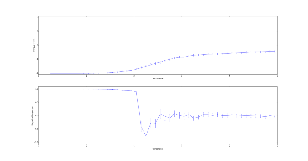
In order to calculate the size of error bars the following formula was used
and the plot function was replaced with the errorbar function. Furthermore since the number of cycles over which the average is taken is stored in a separate class attribute, this was set to reset along with all the others (E,E2, M, etc).
from IsingLattice import *

from matplotlib import pylab as pl

import numpy as np

n_rows = 8

n_cols = 8

il = IsingLattice(n_rows, n_cols)

il.lattice = np.ones((n_rows, n_cols))

spins = n_rows*n_cols

runtime = 60000

times = range(runtime)

temps = np.arange(0.25, 5.0, 0.1)

energies = []

magnetisations = []

energysq = []

magnetisationsq = []

#create lists for energy and magnetisation errors

energy_errors = []

mag_errors = []

for t in temps:

              for i in times:

                            if i % 100 == 0:
                                          print(t, i)
                            energy, magnetisation = il.montecarlostep(t)
              aveE, aveE2, aveM, aveM2, n_cycles, avging_cycles = il.statistics()

              energies.append(aveE)

              energysq.append(aveE2)

              magnetisations.append(aveM)

              magnetisationsq.append(aveM2)

              energy_errors.append(np.sqrt(aveE2 - (aveE**2))/(np.sqrt(avging_cycles)))

              mag_errors.append(np.sqrt(aveM2 - (aveM**2))/(np.sqrt(avging_cycles)))

              #reset the IL object for the next cycle

              il.E = 0.0

              il.E2 = 0.0

              il.M = 0.0

              il.M2 = 0.0

              il.n_cycles = 0

              il.avging_cycles = 0

fig = pl.figure()

enerax = fig.add_subplot(2,1,1)

enerax.set_ylabel("Energy per spin")

enerax.set_xlabel("Temperature")

enerax.set_ylim([-2.1, 2.1])

magax = fig.add_subplot(2,1,2)

magax.set_ylabel("Magnetisation per spin")

magax.set_xlabel("Temperature")

magax.set_ylim([-1.1, 1.1])

enerax.errorbar(temps, np.array(energies)/spins,yerr = energy_errors)

magax.errorbar(temps, np.array(magnetisations)/spins,yerr = mag_errors)

pl.show()

final_data = np.column_stack((temps, energies, energysq, magnetisations, magnetisationsq))

np.savetxt("8x8.dat", final_data)
The Effect of System Size
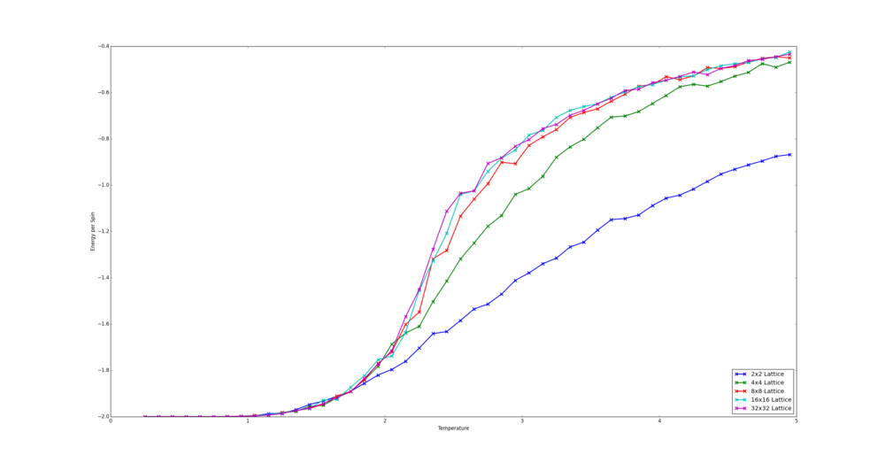
TASK: Repeat the final task of the previous section for the following lattice sizes: 2x2, 4x4, 8x8, 16x16, 32x32. Make sure that you name each datafile that your produce after the corresponding lattice size! Write a Python script to make a plot showing the energy per spin versus temperature for each of your lattice sizes. Hint: the NumPy loadtxt function is the reverse of the savetxt function, and can be used to read your previously saved files into the script. Repeat this for the magnetisation. As before, use the plot controls to save your a PNG image of your plot and attach this to the report. How big a lattice do you think is big enough to capture the long range fluctuations?
Files emailed holding relevant code: effect_of_system_size_plotter_lukas_turcani.py
The simulations were run for the number of steps over which an average is not taken as given by the equation derived earlier plus an additional 60,000 steps. For the 32x32 Lattice the number of steps to be ignored as given by the equation was far too large to be compuationally viable. Therefore the number of steps ignored was double that of the 16x16 lattice. This still allows for a majority of simulations to converge.
The script written places the data saved in the text files into a tuple - the first value holds the data and the second holds the number of spins. This is so that when the lattices are being cycled through, their spin number is easily accesible. All the tuples are placed in a list which is for looped through. The data is extracted using indices, placed into lists holding x and y data and plotted. The smallest size to capture long range fluctuations is likely the 8x8 lattice as it the smallest size to converge to the same energy values as the larger lattices.
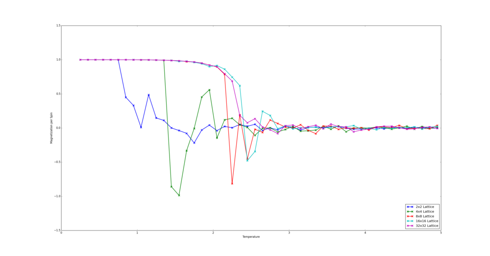
from matplotlib import pylab as plt

import numpy as np

import os as os

#change directory to where files are located

os.chdir("F:\Chemistry\Year 3\Labs\Ising\ImperialChem-Year3CMPExpt-master")

#place the content of each file into a variable - the second entry of the tuple holds the number of spins in the lattice

data_2 = (np.loadtxt("2x2.dat"), 4)

data_4 = (np.loadtxt("4x4.dat"), 16)

data_8 = (np.loadtxt("8x8.dat"), 64)

data_16 = (np.loadtxt("16x16.dat"), 256)

data_32 = (np.loadtxt("32x32.dat"),1024)

lattice_data = [data_2,data_4,data_8,data_16,data_32]

#create graph elements on which energy and magnetisation will be plotted

energy_fig = plt.figure()

energy_ax = energy_fig.add_subplot(111)

mag_fig = plt.figure()

mag_ax = mag_fig.add_subplot(111)

#go through each lattice file 1 by 1

for lattice in lattice_data:

              #make lists which will hold x data - the temperatures and y data - energy / magnetisation

              temps = []

              energies = []

              mags = []

              #each line or "row" hold the energy / magnetisation at a certain temperature - add these to the respective lists

              for row in lattice[0]:

                            temps.append(row[0])

                            energies.append(row[1]/lattice[1])

                            mags.append(row[3]/lattice[1])

              #plot the data

              energy_ax.plot(temps,energies,"-x",lw = 2, ms = 7.5, mew = 2, label = "{0}x{0} Lattice".format(int(np.sqrt(lattice[1]))))

              mag_ax.plot(temps,mags,"-x",lw = 2, ms = 7.5, mew = 2, label = "{0}x{0} Lattice".format(int(np.sqrt(lattice[1]))))

              energy_ax.legend(loc=4)

              mag_ax.legend(loc=4)

              mag_ax.set_ylim([-1.5,1.5])

              energy_ax.set_xlabel("Temperature")

              energy_ax.set_ylabel("Energy per Spin")

              mag_ax.set_xlabel("Temperature")

              mag_ax.set_ylabel("Magnetization per Spin")

plt.show()
Determining the Heat Capacity
Calculating the Heat Capacity
TASK: Write a Python script to make a plot showing the heat capacity versus temperature for each of your lattice sizes from the previous section. You may need to do some research to recall the connection between the variance of a variable, , the mean of its square , and its squared mean . You may find that the data around the peak is very noisy — this is normal, and is a result of being in the critical region. As before, use the plot controls to save your a PNG image of your plot and attach this to the report.
Files emailed holding relevant code: heat_capacity_plotter_lukas_turcani.py
The code in this used here is largely the same as that in the section above. However, the energies list, holding energy per spin data, is replaced with a heat capacities list containing the heat capacity per spin. The values of heat capacity are found with the following formula : . where is the heat capacity.
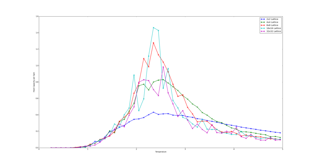
from matplotlib import pylab as plt

import numpy as np

import os as os

#change directory to where files are located

os.chdir("F:\Chemistry\Year 3\Labs\Ising\ImperialChem-Year3CMPExpt-master")

#place the content of each file into a variable - the second entry of the tuple holds the number of spins in the lattice

data_2 = (np.loadtxt("2x2.dat"), 4)

data_4 = (np.loadtxt("4x4.dat"), 16)

data_8 = (np.loadtxt("8x8.dat"), 64)

data_16 = (np.loadtxt("16x16.dat"), 256)

data_32 = (np.loadtxt("32x32.dat"),1024)

lattice_data = [data_2,data_4,data_8,data_16,data_32]

#create graph elements on which heat capacity will be plotted - named energy as edit of previous script

energy_fig = plt.figure()

energy_ax = energy_fig.add_subplot(111)

#go through each lattice file 1 by 1

for lattice in lattice_data:

              #make lists which will hold x data - the temperatures and y data - heat capacity

              temps = []

              heat_capacities = []

              #each line or "row" holds the energy and energy squared at a certain temperature - use these to work out heat capacity and add this to the list

              for row in lattice[0]:

                            temps.append(row[0])

                            heat_capacities.append((row[2] - (row[1]**2))/((lattice[1])*(row[0]**2)))

              #plot the data

              energy_ax.plot(temps,heat_capacities,"-x",lw = 2, ms = 7.5, mew = 2, label = "{0}x{0} Lattice".format(int(np.sqrt(lattice[1]))))

              energy_ax.legend()

              energy_ax.set_xlabel("Temperature")

              energy_ax.set_ylabel("Heat Capacity per Spin")

plt.show()
Locating the Curie Temperature
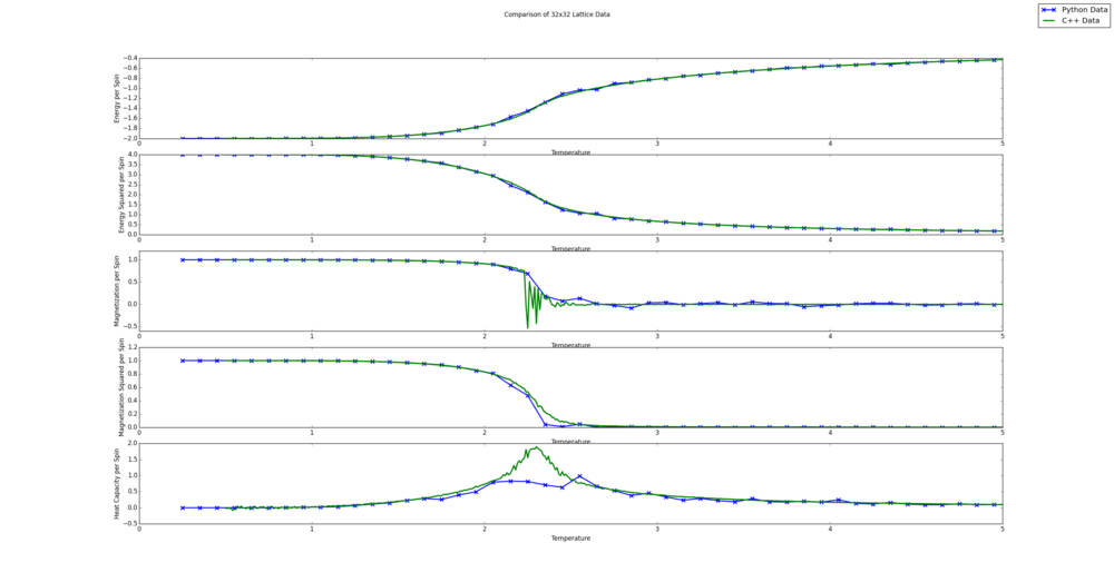
TASK: A C++ program has been used to run some much longer simulations than would be possible on the college computers in Python. You can view its source code here if you are interested. Each file contains six columns: (the final five quantities are per spin), and you can read them with the NumPy loadtxt function as before. For each lattice size, plot the C++ data against your data. For one lattice size, save a PNG of this comparison and add it to your report — add a legend to the graph to label which is which. To do this, you will need to pass the label="..." keyword to the plot function, then call the legend() function of the axis object (documentation here).
File emailed holding relevant code: cpp_comparison_plotter_lukas_turcani.py
The code in this section was very similar to that described in the two sections above, however due to plotting multiple data sets it is slightly more complex. Initially the script is directed to the folder holding the Python data generated in the previous tasks. The loadtxt() function then assigns the data to a variable name. The naming is largely self-explanatory. The script is then redirected to the folder containing the C++ data which is also assigned to appropriately named variables. Since the aim of this exercise is to compare the Python and C++ data for a given lattice size, it is convenient if the two variables containing these data sets were coupled somehow. This is achieved by placing the C++ and Python data containing variables inside a tuple, where the first entry is the Python data, the second entry is the C++ data and the third entry is the spin number for that lattice. The resulting tuples are places in a list.
The use of tuples here increases readability as a single list can be iterated through by a for loop and the necessary data accessed by a simple set of indices. Much easier than the alternative of using multiple lists at once to access the data.
The list of tuples is iterated through by a for loop. Each element, E, of the list corresponds to the set of all data for a given lattice size. This set is made up of 3 subsets - Python data (in index 0), C++ data (index 1), spin number (index 2). At the start of each iteration a figure is created - this holds all the graphs for a given lattice. There are 5 graphs, 1 to compare each quantity between the Python and C++ data sets. The graphs are added to the figure by creating subplots and their axes are labelled. To be able to plot the data it has to be placed in a list. Therefore, a list is created for every quantity to be extracted from E. The Python quantities are extracted from E by using a for loop on index 0 of E. This index holds the Python data in what is essentially a table. The column corresponds to the quantities and the rows correspond to the values of these quantities at different temperatures. Therefore a for loop applied to this index iterates through the table row by row. In each iteration the column is accessed by its index and appended to the corresponding list, after division by the relevant numbers of spins found in index 2 of E. This process is repeated for C++ data by applying a for loop to index 1 of E. Division by spins here is unnecessary as it is already in per spin form.
The list are then plotted using the plot() function.
The resulting figures are shown below. Since the script automatically creates a comparison for all lattices sizes, they are all shown. It is interesting to note that the Python and C++ data seems to agree more for smaller lattice sizes. This is likely because all lattice sizes used the same number of steps to averages values. This leads to a less accurate average value for the bigger lattices as the energy and magnetization values can fluctuate more, due to more degrees of freedom. It is also clear from this comparison that the Python data fails to capture the fluctuations in the magnetization per spin value. This is likely because a fine enough temperature grid was not used.

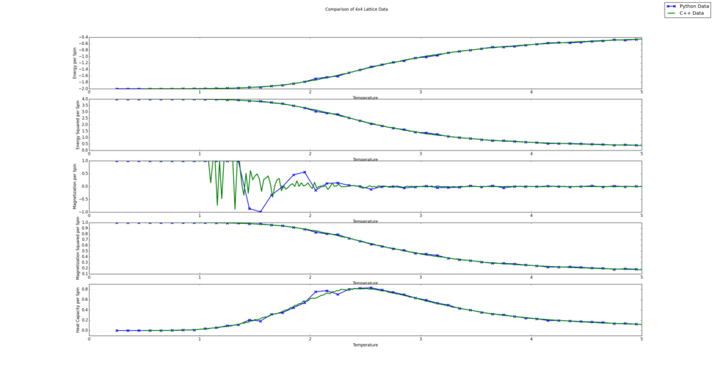

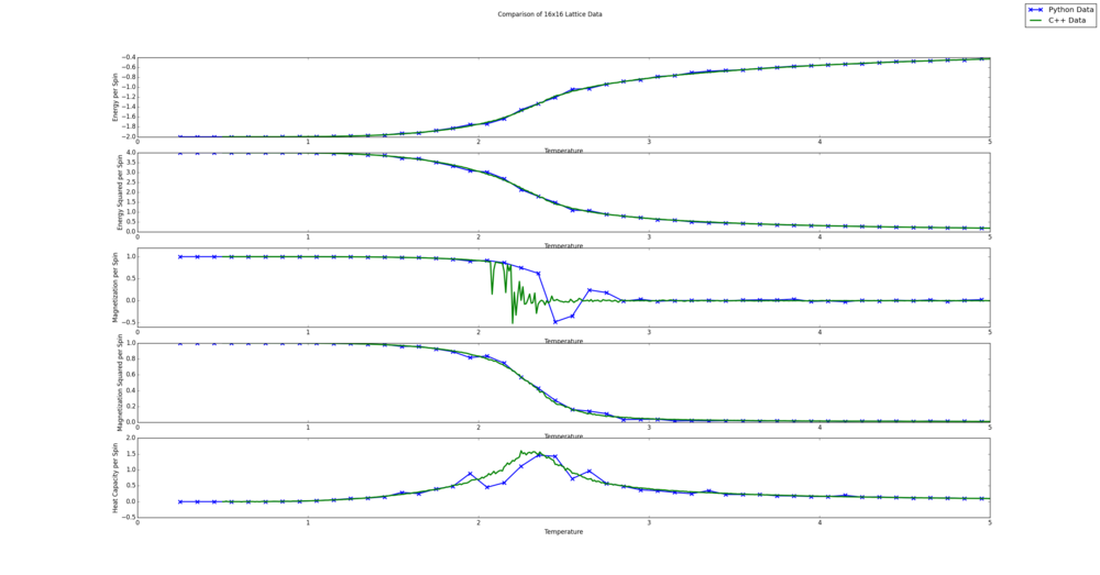
from matplotlib import pylab as plt

import numpy as np

import os as os

#change directory to where files are located

os.chdir("F:\Chemistry\Year 3\Labs\Ising\ImperialChem-Year3CMPExpt-master")

#place the content of each file into a variable

data_2 = np.loadtxt("2x2.dat")

data_4 = np.loadtxt("4x4.dat")

data_8 = np.loadtxt("8x8.dat")

data_16 =np.loadtxt("16x16.dat")

data_32 =np.loadtxt("32x32.dat")

#go to direcotry where C++ data is held

os.chdir("F:\Chemistry\Year 3\Labs\Ising\ImperialChem-Year3CMPExpt-master\C++_data")

#place content into a variable - same idea as above

cpp_2 = np.loadtxt("2x2.dat")

cpp_4 = np.loadtxt("4x4.dat")

cpp_8 = np.loadtxt("8x8.dat")

cpp_16 = np.loadtxt("16x16.dat")

cpp_32 = np.loadtxt("32x32.dat")

#couple the two 2 corresponding data sets to easily cycle through them with for loop - 3rd variable is number of spins

lat_2 = (data_2,cpp_2,4)

lat_4 = (data_4,cpp_4,16)

lat_8 = (data_8,cpp_8,64)

lat_16 = (data_16,cpp_16,256)

lat_32 = (data_32,cpp_32,1024)

#place all data in a list so it can be analysed one by one in a for loop

data_list = [lat_2,lat_4,lat_8,lat_16,lat_32]

for lat in data_list:

              #create figure on which comparison of data points will take place and title it by lattice size

              curr_fig = plt.figure()

              curr_fig.suptitle("Comparison of {0}x{0} Lattice Data".format(int(np.sqrt(lat[2]))))

              #add a set of 5 axes for comparison of energy, magnetisation and heat capacity between the two data sets

              eng_ax = curr_fig.add_subplot(511)

              eng2_ax = curr_fig.add_subplot(512)

              mag_ax = curr_fig.add_subplot(513)

              mag2_ax = curr_fig.add_subplot(514)

              cap_ax = curr_fig.add_subplot(515)

              #label the axes

              eng_ax.set_xlabel("Temperature")

              eng_ax.set_ylabel("Energy per Spin")

              eng2_ax.set_xlabel("Temperature")

              eng2_ax.set_ylabel("Energy Squared per Spin")

              mag_ax.set_xlabel("Temperature")

              mag_ax.set_ylabel("Magnetization per Spin")

              mag2_ax.set_xlabel("Temperature")

              mag2_ax.set_ylabel("Magnetization Squared per Spin")

              cap_ax.set_xlabel("Temperature")

              cap_ax.set_ylabel("Heat Capacity per Spin")

              #extract the data from python generated files and add it to the respective lists so it can be plotted

              py_temps = []

              py_eng = []

              py_eng2 = []

              py_mag = []

              py_mag2 = []

              py_c = []

              for row in lat[0]:

                            py_temps.append(row[0])
                            py_eng.append(row[1] / lat[2])
                            py_eng2.append(row[2] / lat[2]**2)
                            py_mag.append(row[3] / lat[2])
                            py_mag2.append(row[4]/ lat[2]**2)
                            py_c.append((row[2] - (row[1]**2))/((lat[2])*(row[0]**2)))
              #extract the data from C++ generated files and add it to respective list so it can be plotted

              cpp_temps = []

              cpp_eng = []

              cpp_eng2 = []

              cpp_mag = []

              cpp_mag2 = []

              cpp_c = []

              for row in lat[1]:

                            cpp_temps.append(row[0])
                            cpp_eng.append(row[1])
                            cpp_eng2.append(row[2])
                            cpp_mag.append(row[3])
                            cpp_mag2.append(row[4])
                            cpp_c.append(row[5])
              #plot the python and C++ data on the relevant axes

              py_eng_line, = eng_ax.plot(py_temps,py_eng,"-x",lw = 2, mew = 2, ms = 7.5, label = "Python Data")

              cpp_eng_line, = eng_ax.plot(cpp_temps,cpp_eng,lw = 2.5, label = "C++ Data")

              eng2_ax.plot(py_temps,py_eng2,"-x",lw = 2, mew = 2, ms = 7.5, label = "Python Data")

              eng2_ax.plot(cpp_temps,cpp_eng2,lw = 2.5, label = "C++ Data")

              mag_ax.plot(py_temps,py_mag,"-x",lw = 2, mew = 2, ms = 7.5, label = "Python Data")

              mag_ax.plot(cpp_temps,cpp_mag,lw = 2.5, label = "C++ Data")

              mag2_ax.plot(py_temps,py_mag2,"-x",lw = 2, mew = 2, ms = 7.5, label = "Python Data")

              mag2_ax.plot(cpp_temps,cpp_mag2,lw = 2.5, label = "C++ Data")

              cap_ax.plot(py_temps,py_c,"-x",lw = 2, mew = 2, ms = 7.5, label = "Python Data")

              cap_ax.plot(cpp_temps,cpp_c,lw = 2.5, label = "C++ Data")

              plt.figlegend((py_eng_line,cpp_eng_line), ("Python Data", "C++ Data"), loc=1)

              plt.show()
Polynomial Fitting
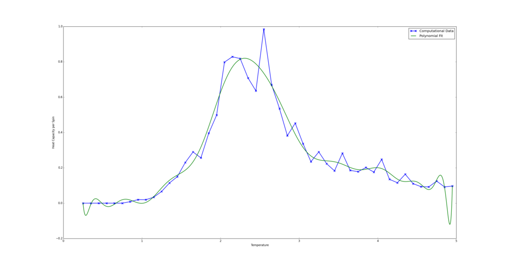
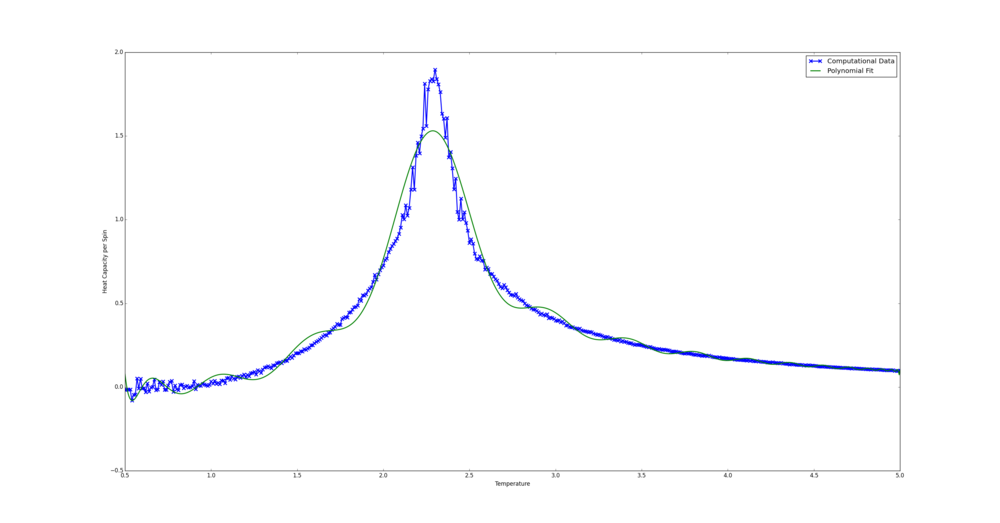
TASK: write a script to read the data from a particular file, and plot C vs T, as well as a fitted polynomial. Try changing the degree of the polynomial to improve the fit — in general, it might be difficult to get a good fit! Attach a PNG of an example fit to your report.
File emailed holding relevant code: heat_capacity_plotter_and_fitter_lukas_turcani.py
The code used in this section was primarily taken from that made available in the instructions. Changes when plotting Python data were (shown in code on wiki):
-inclusion of change directory functions
-addition of variable holding number of spins in the lattice
-The C variable was modified so that it used columns 1,2 and 3 to find the heat capacity through the equation
-the fit was changed from a 3rd to 25th order polynomial
-the data was plotted
When plotting C++ data the changes were the same except the C variable was changed to take the 6th column (shown in script sent via email). Also the Polynomial order was 400.
from matplotlib import pylab as plt

import numpy as np

import os as os

#change directory to where file is located

os.chdir("F:\Chemistry\Year 3\Labs\Ising\ImperialChem-Year3CMPExpt-master")

#number of spins in lattice

spins = 1024.0

data = np.loadtxt("32x32.dat") #assume data is now a 2D array containing two columns, T and C

T = data[:,0] #get the first column

C = (data[:,2]-(data[:,1]**2))/(spins*(data[:,0]**2)) # get the heat capacity

#first we fit the polynomial to the data

fit = np.polyfit(T, C, 25) # fit a 25th order polynomial

#now we generate interpolated values of the fitted polynomial over the range of our function

T_min = np.min(T)

T_max = np.max(T)

T_range = np.linspace(T_min, T_max, 1000) #generate 1000 evenly spaced points between T_min and T_max

fitted_C_values = np.polyval(fit, T_range) # use the fit object to generate the corresponding values of C

plt.plot(T,C,"-x",lw=2,mew=2,ms=7.5,label="Computational Data")

plt.plot(T_range,fitted_C_values,lw=2,label="Polynomial Fit")

plt.ylabel("Heat Capacity per Spin")

plt.xlabel("Temperature")

plt.legend()

plt.show()
Fitting in a Particular Temperature Range
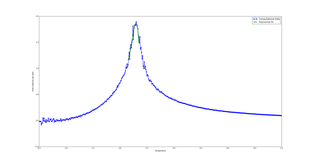
TASK: Modify your script from the previous section. You should still plot the whole temperature range, but fit the polynomial only to the peak of the heat capacity! You should find it easier to get a good fit when restricted to this region.
File emailed holding relevant code: heat_capacity_plotter_and_fitter_MOD_lukas_turcani.py
The bulk of the code here was once again generously provided. In the Python case the curve was fit in the temperature range 1.9-2.8. This was chosen as by eye it seems to be where the peak is steepest. The Python fit code is shown below.
In the C++ case the range chosen was 2.15-2.35. This was on the bases of the fit curve sitting snugly on the computational data. A polynomial of order 5 seemed to produce are reasonable fit. This version of the code was emailed.

from matplotlib import pylab as plt

import numpy as np

import os as os

#change directory to where file is located

os.chdir("F:\Chemistry\Year 3\Labs\Ising\ImperialChem-Year3CMPExpt-master")

#number of spins in lattice

spins = 1024.0

data = np.loadtxt("32x32.dat") #assume data is now a 2D array containing two columns, T and C

T = data[:,0] #get the first column

C = (data[:,2]-(data[:,1]**2))/(spins*(data[:,0]**2)) # get the second column

Tmin = 1.9

Tmax = 2.8

selection = np.logical_and(T > Tmin, T<Tmax)

peak_T_values = T[selection]

peak_C_values = C[selection]

#first we fit the polynomial to the data

fit = np.polyfit(peak_T_values, peak_C_values, 3) # fit a 3rd order polynomial

#now we generate interpolated values of the fitted polynomial over the range of our function

T_min = np.min(T)

T_max = np.max(T)

T_range = np.linspace(Tmin, Tmax, 1000) #generate 1000 evenly spaced points between T_min and T_max

fitted_C_values = np.polyval(fit, T_range) # use the fit object to generate the corresponding values of C

plt.plot(T,C,"-x",lw=2,mew=2,ms=7.5,label="Computational Data")

plt.plot(T_range,fitted_C_values,lw=2,label="Polynomial Fit")

plt.ylabel("Heat Capacity per Spin")

plt.xlabel("Temperature")

plt.legend()

plt.show()
Finding the Peak in C
TASK: find the temperature at which the maximum in C occurs for each datafile that you were given. Make a text file containing two colums: the lattice side length (2,4,8, etc.), and the temperature at which C is a maximum. This is your estimate of for that side length. Make a plot that uses the scaling relation given above to determine . By doing a little research online, you should be able to find the theoretical exact Curie temperature for the infinite 2D Ising lattice. How does your value compare to this? Are you surprised by how good/bad the agreement is? Attach a PNG of this final graph to your report, and discuss briefly what you think the major sources of error are in your estimate.
File emailed holding relevant code: heat_capacity_plotter_and_fitter_MOD_lukas_turcani.py + curie_plotter_lukas_turcani.py
The lines
Cmax = np.max(fitted_C_values)

Tmax = T_range[fitted_C_values == Cmax]
were added at the bottom of the code from the above task. The table of the results is shown below
| Lattice Side Length | TC |
|---|---|
| 2 | 2.5018018 |
| 4 | 2.44414414 |
| 8 | 2.33723724 |
| 16 | 2.30621622 |
| 32 | 2.29854855 |
| 64 | 2.25527027 |
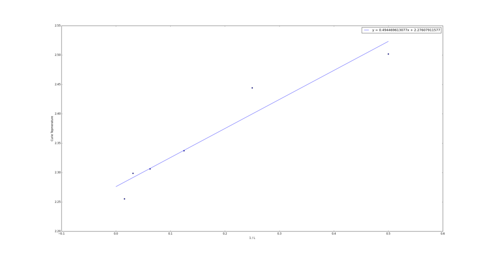
The Curie Temperature for an infinite 2D lattice estimated here is 2.276 J. This is remarkably close to the theoretical limit as the size of the lattice approach infinity at 2.269 J1 . The major source of error here is likely to be the fitting. There are two components to this, firstly selecting an order for the polynomial and secondly picking the temperature range.
from matplotlib import pylab as plt

import numpy as np

#list of curie temperature

tc = [2.5018018,2.44414414,2.33723724,2.30621622,2.29854855,2.25527027]

#list of inverse side lengths

inv_l = [(1.0/2.0),(1.0/4.0),(1.0/8.0),(1.0/16.0),(1.0/32.0),(1.0/64.0)]

#fit data to first order polynomial

fit = np.polyfit(inv_l, tc,1)

 #generate 1000 evenly spaced points between 0 and max(inv_l)

l_range = np.linspace(0, max(inv_l), 1000)

fitted_C_values = np.polyval(fit, l_range)

#plot

plt.scatter(inv_l,tc)

plt.plot(l_range,fitted_C_values,label = "y = {0}x + {1}".format(fit[0],fit[1]))

plt.xlabel("1 / L")

plt.ylabel("Curie Tepmerature")

plt.legend()

plt.show()
NJ: that's true — how sensitive is the position of the maximum to these two choices? You could also ignore the very small lattices, since they are likely to be the noisiest data.
NJ: very good work overall. If I could make a general suggestion, it would be to try to change your comments from an exact description of what each python command does to a more general overview of what's going on. The idea is that if you come back to these files after months or years, you'll still know what the Python commands mean, but your thought process at the time you wrote them might not be so clear.
References
http://micro.stanford.edu/~caiwei/me334/Chap12_Ising_Model_v04.pdf


