Talk:Mod:lnwliqsim

JC: General comments: Good report with clear explanations of your results and some background research. Make sure that you fully understand the system that you are working with.

Simulation of a Simple Liquid

Theory

Classical Particle Approximation

The Schrödinger equation can be use to describe the behaviour of chemical systems. However it can only be solved accurately for a single hydrogen atom. To approximate a larger system, a classical particle theory can be applied. For a system of N atoms, each atom will interact with every other atom in the system. The force felt by each can be used to detemine the velocity with which it is moving.

$F_i=m_i{\mathbf{a}}_i=m_i\frac{d{\mathbf{v}}_i}{dt}=m_i\frac{d^2{\mathbf{x}}_i}{d{t}^2}$

For N atoms, N equations are needed to describe the system. The Verlet alogrithm is used to help solve these systems of equations, by comparing the Taylor expansion of the position of a particle $x_i$ both forward and backwards it time to get.

${\mathbf{x}}_i(t+\delta t)\approx 2{\mathbf{x}}_i(t)-{\mathbf{x}}_i(t-\delta (t))+\frac{{\mathbf{F}}_i(t)\delta t^2}{m_i}$

However, the velocity cannot be determined using this method, therefore another version of the Verlet algorithm known as the Velocity Verlet Algorithm is used instead. This works by taking the acceleration into account, and considering half time steps, $\frac{1}{2}\delta (t)$.

${\mathbf{v}}_i(t+\delta t)={\mathbf{v}}_i(t+\frac{1}{2}\delta t)+\frac{1}{2}{\mathbf{a}}_i(t+\delta t)\delta t$

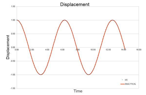
From the time, the clasical analytical value of displacement was calculated using

$x(t)=Acos(\omega t+\varphi )$

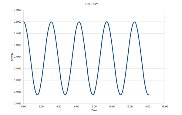
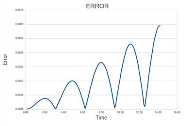
and the error was found by finding the difference between the classical value and the position value determined by the Verlet algorithm. The total energy of the system was found by summing the kinetic and potential energies of the Verlet system.

$E_{tot}=\frac{1}{2}m{\mathbf{v}}^2+\frac{1}{2}k{\mathbf{x}}^2$

Figure (1). Graphs showing the Velocity and Energy of the Verlet Velocity Algorithm.

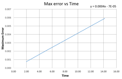
As seen in Fig. (1) and (2), the error increases with every oscillation, and what can appear a small error is carried forward with every iteration and the error is compounded. This is because the two systems are slightly out of phase with each other and so as the silution progresses this difference has a larger and larger effect on the relationship between them.

Figure (2). Graphs showing Error of the Verlet Velocity compared to the Classical Solution.

Figure (3). Percentage Energy Difference over the whole system against value of Time Step

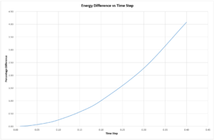
The energy difference of the system over time was plotted against changing values of the time step, see fig. (3). A value for the time step less that 0.20 ensured that the energy difference between the maximum and minimum for a system was not more than 1%. The energy of an isolated system should be monitored during simulation to ensure that energy is conserved.

JC: Good analysis of the timestep dependence. Which timesteps did you try? Plot the data points in figure 3 rather than a smooth line.

Lennard Jones Potential

The force acting on an object is determined by the potential it experiences:

${\mathbf{F}}_i=-\frac{dU({\mathbf{r}}^N)}{d{\mathbf{r}}_i}$

For many simple systems the same potential can be applied. The Lennard Jones curve contains a large repulsive potential at small separations and a harmonic potential close to equilibrium, with the form:

$U({\mathbf{r}}^N)=\sum _i^N\sum _{i\ne j}^{N}4ϵ(\frac{{\sigma }^{12}}{r_{ij}^{12}}-\frac{{\sigma }^6}{r_{ij}^6})$

For a single Lennard Jones interaction, $\varphi (r)=4ϵ(\frac{{\sigma }^{12}}{r_{ij}^{12}}-\frac{{\sigma }^6}{r_{ij}^6})$, $\varphi (r)=0$ occurs when $r_0=\sigma$. The force experienced at this separation is found by differentiating the potential.

${\mathbf{F}}_i(r_0)={\varphi }^{\prime }(r_0)=\frac{-24ϵ}{r_0}(2\frac{{\sigma }^{12}}{r_0^{12}}-\frac{{\sigma }^6}{r_0^6})$

${\mathbf{F}}_i=\frac{-24ϵ}{\sigma }$

JC: The result is correct, but the differentiation in the previous line isn't right.

The equilibrium value of for position, $r_{eq}$, is found by considering ${\mathbf{F}}_i=0$.

${\mathbf{F}}_i(r_0)=\frac{-24ϵ}{r_0}(2\frac{{\sigma }^{12}}{r_0^{12}}-\frac{{\sigma }^6}{r_0^6})=0$

$\frac{2{\sigma }^{12}}{r^{12}}=\frac{{\sigma }^6}{r^6}$

$r_{eq}=2^{\frac{1}{6}}\sigma$

The well depth, $\varphi (r_{eq})$, gives an idea of the strength of interaction between the two particles.

$\varphi (r_{eq})=4ϵ(\frac{{\sigma }^{12}}{(2^{\frac{1}{6}}\sigma {)}^{12}}-\frac{{\sigma }^6}{(2^{\frac{1}{6}}\sigma {)}^6})$

$\varphi (r_{eq})=4ϵ(\frac{1}{4}-\frac{1}{2})=-ϵ$

Integral of the potential curve gives the total energy of all particles in the system under the curve to the point. By integrating from a cut-off to infinity, the interaction energy of all particles with an inter-atomic separation larger than the cut off point is calculated.

$\underset{x}{\overset{\mathrm{\infty }}{\int }}\varphi (r)d\mathbf{r}=\underset{x}{\overset{\mathrm{\infty }}{\int }}4ϵ(\frac{{\sigma }^{12}}{r_{ij}^{12}}-\frac{{\sigma }^6}{r_{ij}^6})d\mathbf{r}$

$\underset{x}{\overset{\mathrm{\infty }}{\int }}\varphi (r)d\mathbf{r}={[\frac{-4{\sigma }^{12}}{11r^{11}}+\frac{4{\sigma }^6}{5r^5}]}_x^{\mathrm{\infty }}$

x	Evaluation of Integral
$2\sigma$	−0.0248
$2.5\sigma$	−0.00873
$3\sigma$	−0.00329

JC: Correct.

LAMMPS

The liquid simulations were run using LAMMPS, Large-scale Atomic/Molecular Massively Parallel Simulator. LAMMPS is a classical molecular dynamics code used to model atoms, particle systems and polymers under different conditions. It can run several different simulations in parallel from one script. LAMMPS can be programmed to calculate and record data points of many different system variables.

Periodic Boundary Conditions

Realistic volumes of liquid contain many moles of particles which cannot be reasonably simulated even with vast amounts of computational power. In 1 mL of water, there are $3.342\times 10^{22}$ molecules. For a reasonable simulation, around 1000-10,000 molecules are simulated. Again considering water, the volume of 10,000 molecules is $2.99\times 10^{-20}$ mL, far smaller than any real world system.

JC: The volume of 10000 molecules should be 2.99 x 10^-19 so you're out by a factor of 10. Show your working for these calculations.

To simulate a bulk liquid, the unit cell that is considered is imagined to be replicated in every direction. This means that as one particle leaves one edge of the main box, it re-enters through the opposite edge. For example an atom that starts at $(0.5,0.5,0.5)$ and moves $(0.7,0.6,0.2)$ during the course of the simulation, ends up at $(0.2,0.1,0.7)$ after application of the boundary conditions.

JC: Correct.

Truncation

Due to the replication of every particle in the infinite cells in every direction, the number of interactions of the particles must be controlled. This is done by setting a distance, $\mathbf{x}$, at which the interaction energy (measured by the area under the Lennard-Jones potential) is small enough to be considered neglible, and thus can be ignored.

Reduced Units

When working with the Lennard Jones Potential, reduced units are often used. This is done to make values more managable, no longer having to deal with power terms, instead numbers near unity. For the rest of this report, only reduced units are used.

Parameter	Formula
distance	$r*=\frac{r}{\sigma }$
energy	$E*=\frac{E}{epsilon}$
temperature	$T*=\frac{k_{B}T}{ϵ}$

For argon, $\sigma =0.34nm$ $\frac{ϵ}{k_B}=120K$, the Lennard-Jones cut-off is $r*=3.2$.

In real units this cut off is equal to

$r=r*\times \sigma =3.2\times 0.34nm=1.088nm$

The well depth in real units is equal to

$E_{welldepth}=E{*}_{welldepth}\times ϵ$

$E_{welldepth}=-1\times (120\times k_B)=-1.657\times 10^{-21}J=1.005kJmo{l}^{-}1$

and the temperature when $T*=1.5$, is

$\frac{T*ϵ}{k_B}=T=180K$

JC: Correct, but give your answers to the same number of significant figures as used in the question (in this case 2).

Equilibration

The same script was run at 5 different time steps to determine the effect of the time steps on the outcome of the simulation. A crystal lattice is generated, then melted to simulate a liquid-like structure. Atoms are not generated with random starting coordinates as they could end up being too close together and giving the energy value of the system an abnormally high value due to the strength of their interaction.

JC: A simulation starting from a configuration with high repulsion is likely to be unstable and to crash unless a much smaller timestep is used.

The lattice is 'built' in the script with a simple cubic structure and a number density of 0.8. The output file gives us the lattice spacing

 Lattice spacing in x,y,z = 1.07722 1.07722 1.07722 

These two values both correspond to the same lattice.

The volume of the cell is

$1.07722^3=1.25$

and the number density is given by

$\frac{1}{vo{l}_{cell}}=\frac{1}{1.25}=0.8$

JC: What about the side length of an fcc lattice?

A block of 10 x 10 x 10 unit cells is created and 1000 atoms created to fill the whole system, from the command

 create_atoms 1 box 

As this lattice has been defined as a simple cubic lattice it containes only 1 lattice point per cell. For a face centered cubic lattice, there are 4 lattice points per unit cell, if this same command was used to create atoms to fill a fcc lattice, would generate not 1000 atoms but 4000.

JC: Correct.

Setting the properties of atoms

A script used to define the properties of the atoms is given below.

 mass 1 1.0 
pair_style lj/cut 3.0
pair_coeff * * 1.0 1.0 

The first command mass sets the mass of the atom type. This would give all atoms of type 1 a mass of 1.0.

The command pair_style defines the pairwise interactions felt by the particles. In this case, the standard 12/6 Lennard-Jones potential is computed. It also defines the cutoff point given by cut at which interaction energies are considered negligible.

Pair_coeff defines he pairwise force field coefficients felt by pairs of atoms. The * defines this for all atoms in the system. The last two arguments are parameters for $ϵ$ and $\sigma$ respectively.

JC: Good understanding.

The velocity of each atoms is then specified in the script.

 velocity all create 1.5 12345 dist gaussian rot yes mom yes 

By using the command all, all atoms in the simulation will be assigned a velocity. Create 1.5 12345 dist gauss tells the program to generate an array of velocities with a random number generator, at a specified temperature, using a gaussian distribution. The linear and angular momentums of the velocities is set to 0 by mom yes rot yes.

As both the position ${\mathbf{x}}_i$ and velocity ${\mathbf{v}}_i$ are specified the Verlet Velocity Algorithm is used.

JC: What would be needed for the standard Verlet algorithm to be used.

Running the simulation

### SPECIFY TIMESTEP ###
variable timestep equal 0.001
variable n_steps equal floor(100/${timestep})
variable n_steps equal floor(100/0.001)
timestep ${timestep}
timestep 0.001

### RUN SIMULATION ###
run ${n_steps}
run 100000

The command varible timestep equal 0.001 logs a value of 0.001. If the word 'timestep' appears on subsequent lines in a function , ${}, then this string is replaced by the value, 0.001. This could also be written

timestep 0.001
run 100000

However, if the timestep is to be varied, the top script makes it much quicker to change, only having to edit one line. In the second script, every term containing the timestep would need to be edited individually.

Figure (4). Graphs of Energy, Pressure and Temperature against time for 0.001 system.

Energy	Pressure	Temperature

Figure (5). Energy vs Time for each value of time step

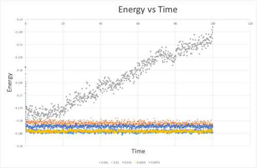
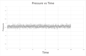
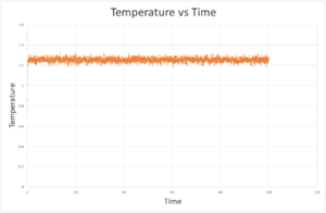
The energy against time for 5 different time steps is plotted in figure (5). The time step 0.01 is too large a time step, and causes an error due to the nature of the verlet algorithm which is compounded with each step. Although both 0.01 and 0.0075 both reach equilibrium, they give a slightly more positive value of the energy than 0.0025 and 0.001 both give similar energies, and also reach equilibrium. The value of the time step is a compromise between the a short step to give accurate values compared to reality and a larger step in order to cover a longer period of time for a given number of iterations of the program. As a balance between accuracy and length of simulation 0.0025 gives the most acceptable results.

JC: Good choice of timestep. Why is it a problem that timesteps of 0.01 and 0.0075 give simulations with higher energies? Should energy depend on timestep?

Simulations under Specific conditions

The microcanonical ensemble was used in previous simulations, which keeps the number of particles, the volume of the system and the total energy of the system constant. However, this is not very useful to simulate chemical systems, which often operate under constant pressure. For this the isobaric-isothermal ensemble, NpT, can be used. The program runs by 'melting' a crystal lattice, but defines different thermodynamic variables to keep constant in the system.

variable T equal ...
variable p equal ...
variable timestep equal ...

The temperature of the system is kept contant during the simulations using the equipartion theorum. By equating the energy from the equipartition theorum with the kinetic energy

$E_k=\frac{3}{2}N{k}_{B}T=\frac{1}{2}\sum _i{m}_i{v}_i^2$

the instantaneous temperature,

$T$

, of the system is calculated. The instantaneous temperature will fluctuate as the simulation proceeds, so it keep the temperature at the preset temperature,

$\mathfrak{𝔗}$

, the velocity is premultiplied by a factor

$\gamma$

.

$\gamma$

is found by comparing

$\frac{1}{2}\sum _i{m}_i{v}_i^2=\frac{3}{2}N{k}_{B}T$ (1) $\frac{1}{2}\sum _i{m}_i{\left(\gamma v_i\right)}^2=\frac{3}{2}N{k}_B\mathfrak{𝔗}$ (2)

and solving for $\gamma$. By dividing (2) by (1), gamma is found to be $\gamma =\sqrt{\frac{\mathfrak{𝔗}}{T}}$

JC: Correct.

fix aves all ave/time 100 1000 100000 v_dens v_temp v_press v_dens2 v_temp2 v_press2
run 100000

The code above generates an average over the entire system. The three numbers 100 1000 100000 determine the range over which the average will be taken. After 100,000 steps (i.e. the end of the simulation), 1000 values are averaged, with the values being sampled from every 100 timesteps. For a run of 100000 timesteps with a timestep of 0.0025 the total duration of the simulation will be 250 seconds.

Plotting Equations of State

Simulations were run for 5 different temperatures at

Figure (6). Graph of density against Temperature, with comparison to the Ideal Gas Law.

• 1.55
• 1.75
• 1.95
• 2.15
• 2.35

with at two different pressures, 2.5 and 3.0.

JC: Why do you use a polynomical fit for the ideal gas data point? You know the equation that relates density to temperature for the ideal gas.

The graphs of density against time temperature for the two different pressures were plotted, see fig. (6), and compared to the theoretical density from the Ideal Gas Law. The simulated density was much lower than the density predicted using the Ideal Gas Law. This is because one of the assumptions made when using the Ideal Gas Law, is that there are no interactions between molecules. In the Lennard-Jones potential there is a large repulsive force experience when the inter-nuclear separation becomes too small, but this is not present in the Ideal Gas model. This means that atoms can pack together as close as their radius allows without any energy penalties, unlike a real system where electrostatic repulsions would prevent this. At $T=0$, the density in the Ideal Gas model would be infinite. However, at higher values of temperature, the discrepancy between the two models decreases.

JC: How well does the ideal gas law agree with the simulations at different pressures?

Heat Capacities using Statistical Physics

Heat capacity is the amount of energy required to heat a system by a given temperature. It can be found by

$C_V=\frac{\partial U}{\partial T}=\frac{Var[E]}{k_B{T}^2}=N^2\frac{⟨E^2⟩-⟨E{⟩}^2}{k_B{T}^2}$

where Var[E] is the variance in the energy. The factor of $N^2$ is required to correct the output to the total energy, rather than the energy per particle which is what is automatically generated by LAMMPS.

As before, a crystal is built and then melted, and the density of the crystal is changed by varying the lattice parameter.

 lattice sc ... 

Unlike previously, where we worked in the NpT ensemble, to calculate the heat capacity the NVT ensemble must be used, which was done as seen below.

 variable tdamp equal ${timestep}*100
fix nvt all nvt temp ${T} ${T} ${tdamp}
run 10000
unfix nvt
fix nve all nve
reset_timestep 0

The script for the calculation of the heat capacity is shown below. After the all the data has been collected for each value of the time step, the heat capacity is worked out using the averages shown above.

variable aveenergy equal f_aves[1]
variable avetemp equal f_aves[2]
variable aveenergy2 equal f_aves[3]
variable heatcapacity equal atoms*atoms*(v_aveenergy2-v_aveenergy*v_aveenergy)/(v_avetemp*v_avetemp)
variable heatcpvol equal atoms*atoms*(v_aveenergy2-v_aveenergy*v_aveenergy)/(v_avetemp*v_avetemp*vol)

The an example full script can be found here.

Figure (7). Heat Capacity per Volume against Temperature for two different densities

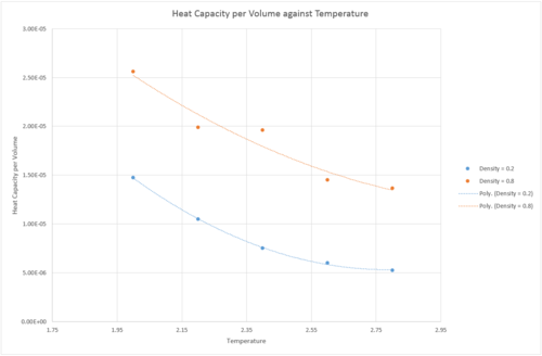
Ten simulations were run, at two densities, 0.2 and 0.8 and 5 temperatures, 2.0, 2.2, 2.4, 2.6 and 2.8. $\frac{C_V}{V}$ was plotted as a function of temperature. As seen in fig. (7), the heat capacity decreases with increased temperature for both systems. Heat capacity is defined as $C_V=\frac{\partial U}{\partial T}$. It would be expected that the heat capacity of the system increased with temperature as the rotational and vibrational energy levels become accessible at higher temperatures, and contribute to the internal energy of the system, increasing the heat capacity. However, this is not seen in the simulation. This is due to the system crossing the Frenkel line, and moving from a relatively rigid vibrational mode into a more diffuse gas like system . This causes less vibration with increased temperature but more diffusion, leading to a lower internal energy. The system with the lower density has a lower heat capacity per volume. This is expected as heat capacity is an extensive property, so a system with more atoms (for example, a higher density) would have a larger heat capacity.

JC: The simulation is of spherical particles, so there is no rotational or vibrational energy levels. Good explanation of the effect of density and good research from the literature for the trend with temperature.

Structural Properties and the Radial Distribution Function

The radial distribution function of a liquid system is very useful. It can be used to determine many different properties of the system, including the structure and parameters of the lattice. The radial distriubtions, and running integrals, of solid, liquid and vapour phases of a Lennard-Jones fluid were simulation using VMD. The densities and temperature were determined using fig (8).

Figure (8). Coexistance curve of Lennard-Jones Fluid

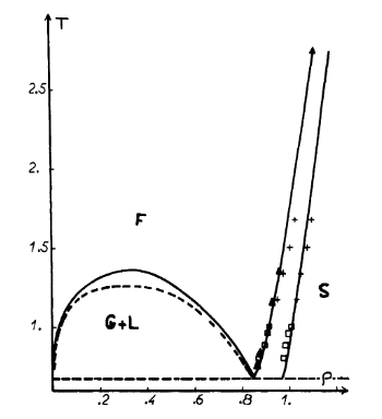
Phase	Density	Temperature
Solid	1.2	1.5
Liquid	0.85	1
Vapour	0.01	1

The RDFs for the three phases are all identical until from r = 0 to r = 0.875. This is due to the strong repulsive potential experienced at short distances. The RDF of the vapour phase has only one peak at r = 1.125. A large peak occurs around this value for all three phases. The liquid RDF has peaks several peaks that oscillate around 1 with the amplitude decaying exponentially as r increases. This indicates some short range order in the liquid, although no long range, with 3 or 4 shells of atoms surrounding the considered atom.

Figure (9). Radial Distribution Functions of solid, liquid and vapour states.

The RDF of the solid reflects the structure of the lattice. Due to the long range order of the solid, there is structure to the RDF far from the atom, although the peaks broaden due to fluctuations in the atom positions.

JC: Good understanding of the RDFs for the different phases.

For te solid, the lattice spacing can be determined from the positions of the peaks. As seen in fig. (10)

Figure (10). Schematic showing nearest neighbors on face centered cubic lattice.

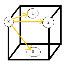
, the first peak corresponds to an shell of nearest neighbors in the middle of the adjacent face, where

$r_1=r_l\times cos(\frac{\pi }{4})$

To find the lattice spacing, $r$

$r_{lat}=\frac{r_1}{cos(\frac{\pi }{4})}=\frac{1.03}{cos(\frac{\pi }{4})}=1.45$

Alternatively the distance to the 2nd nearest neighbor should also give the lattice spacing.

$r_{lat}=r_2=1.48$

Therefore the lattice spacing must lie somewhere between these two values, depending on the uniformity and degree of vibration in the lattice. From theory, for a fcc lattice, the lattice spacing can be found by $$\begin{gathered} r_{lat}=\sqrt[3]{\frac{lattice \\ points}{number \\ density}}=\sqrt[3]{\frac{4}{1.2}}=1.49 \end{gathered}$$.

JC: Good idea to compare the lattice spacing calculated from the different peaks of the solid RDF. What spacing does the 3rd peak predict? Can you suggest any reasons why the lattice spacing predicted from each peak is slightly different?

Figure (11). Running integral of Radial Distribution Function for face centered cubic solid

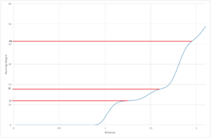
The number of nearest neighbors is determined from the running integral, fig (11). These values agree with a face centered cubic structure.

Nearest Neighbor	Integral Range	Coordination number
1	0 - 12	12
2	12-18	6
3	18 - 42	24

Dynamical Properties and the diffusion coefficient

Mean Squared Displacement

The mean squared displacement of a particle is the average deviation of a particle with reference to a standard position over time.

$MSD=⟨(x-x_0{)}^2⟩=\frac{1}{T}\sum _{t=1}^T(x(t)-x_0{)}^2$

Simulations for 8,000 atoms were run to determine the mean square displacement, and then compared to systems simulated with 1,000,000 atoms.

Phase	Density	Temperature
Solid	1.2	1.5
Liquid	0.8	1.2
Vapour	0.05	1

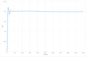
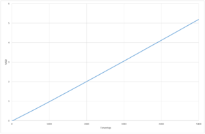
The resultant plots of mean squared displacement are as expected. The solid simulations reach a constant value of displacement after equilibration, as solids do not experience Brownian motion. Both the liquid and the vapour mean square displacements increase with time, as they undergo movement in their fluid states. The solid

Figure (12). Plots of Mean Squared Displacement for three phases.

	8,000 molecules	1,000,000 molecules
solid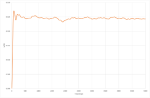
liquid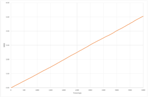
vapour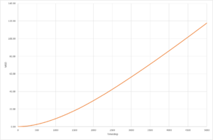

The diffusion coefficient, $D$ is found by

$D=\frac{1}{6}\frac{\partial ⟨r^2(t)⟩}{\partial t}$

By taking the derivative of the MSD after the system has equilibrated, the diffusion coefficient is found to be

	Diffusion Coefficient
	8,000 molecules	1,000,000 molecules
solid	$-2.82\times 10^{-7}{s}^{-1}$	$-8.43\times 10^{-6}{s}^{-1}$
liquid	$8.49\times 10^{-2}{s}^{-1}$	$8.73\times 10^{-2}{s}^{-1}$
vapour	$2.55s^{-1}$	$3.13s^{-1}$

The calculated value for the solid for both simulations is so low, that it can be assumed that diffusion does not occur. The plot for the liquid system appears to be a straight line,and only has a very small non-linear region so the gradient can be determined over the whole range of time step, whereas for the solid and vapour the diffusion coefficient can only be determined from the region of the graph with a constant gradient as they have much larger non-linear regions. The values of diffusion coefficient calculated by the 1,000,000 system are higher than those calculated from the 8,000 molecule system. The simulations with 1,000,000 molecules appear to have reached a more stable value of equilibrium, due to the increased number of molecules in the system.

JC: Show graphs with the fits that you used to obtain the diffusion coefficients. Why do you think there is a difference between the larger and smaller systems, are they at the same densities?

Velocity Autocorrelation Function

The diffusion coefficient can be calculated using the velocity autocorrelation function,

$C(\tau )=⟨\mathbf{v}(t)\cdot \mathbf{v}(t+\tau )⟩$

This function is able to show us how different an atom will be at time $t+\tau$ and time $t$ . An atoms velocity at large values of time should not depend on its velocity at small values of time. The diffusion coefficient can be found by integrating $C(\tau )$ at time, $t=0$.

Using the 1D harmonic oscillator model,

$x=Acos(\omega t+\varphi )$

$v(t)=-A\omega sin(\omega t+\varphi )$

and substituting into $C(\tau )$

$C(\tau )=\frac{\underset{-\mathrm{\infty }}{\overset{\mathrm{\infty }}{\int }}v(t)v(t+\tau )dt}{\underset{-\mathrm{\infty }}{\overset{\mathrm{\infty }}{\int }}{v}^2(t)dt}$

$C(\tau )=\frac{\underset{-\mathrm{\infty }}{\overset{\mathrm{\infty }}{\int }}-A\omega sin(\omega t+\varphi )\cdot -A\omega sin(\omega (t+\tau )+\varphi )dt}{\underset{-\mathrm{\infty }}{\overset{\mathrm{\infty }}{\int }}(-A{)}^2{\omega }^{2}si{n}^2(\omega t+\varphi )dt}$

$C(\tau )=\frac{\underset{-\mathrm{\infty }}{\overset{\mathrm{\infty }}{\int }}sin(\omega t+\varphi )\cdot sin(\omega (t+\tau )+\varphi )dt}{\underset{-\mathrm{\infty }}{\overset{\mathrm{\infty }}{\int }}si{n}^2(\omega t+\varphi )dt}$

Substitutions can be used to simplify the integral

$\alpha =\omega t+\varphi$

$\beta =\omega \tau$

$dt=\frac{1}{\omega }d\alpha$

The integral then becomes

$C(\tau )=\frac{\underset{-\mathrm{\infty }}{\overset{\mathrm{\infty }}{\int }}sin(\alpha )\cdot sin(\alpha +\beta )d\alpha }{\underset{-\mathrm{\infty }}{\overset{\mathrm{\infty }}{\int }}si{n}^2(\alpha )d\alpha }$

$C(\tau )=\frac{\underset{-\mathrm{\infty }}{\overset{\mathrm{\infty }}{\int }}sin(\alpha )\cdot sin(\alpha )cos(\beta )+sin(\alpha )\cdot cos(\alpha )sin(\beta )d\alpha }{\underset{-\mathrm{\infty }}{\overset{\mathrm{\infty }}{\int }}si{n}^2(\alpha )d\alpha }$

$C(\tau )=\frac{\underset{-\mathrm{\infty }}{\overset{\mathrm{\infty }}{\int }}sin(\alpha )\cdot sin(\alpha )cos(\beta )}{\underset{-\mathrm{\infty }}{\overset{\mathrm{\infty }}{\int }}si{n}^2(\alpha )d\alpha }+\frac{\underset{-\mathrm{\infty }}{\overset{\mathrm{\infty }}{\int }}sin(\alpha )\cdot cos(\alpha )sin(\beta )d\alpha }{\underset{-\mathrm{\infty }}{\overset{\mathrm{\infty }}{\int }}si{n}^2(\alpha )d\alpha }$

Consider the first term,

$C(\tau )=\frac{\underset{-\mathrm{\infty }}{\overset{\mathrm{\infty }}{\int }}sin(\alpha )\cdot sin(\alpha )cos(\beta )}{\underset{-\mathrm{\infty }}{\overset{\mathrm{\infty }}{\int }}si{n}^2(\alpha )d\alpha }$

$cos(\beta )$ can be taken out of the equation as it is constant, we then get

$C(\tau )=cos(\beta )\frac{\underset{-\mathrm{\infty }}{\overset{\mathrm{\infty }}{\int }}si{n}^2(\alpha )}{\underset{-\mathrm{\infty }}{\overset{\mathrm{\infty }}{\int }}si{n}^2(\alpha )d\alpha }=cos(\beta )\times 1=cos(\beta )$

Now considering the second term, we can remove the constant from the denominator,

$C(\tau )=sin(\beta )\frac{\underset{-\mathrm{\infty }}{\overset{\mathrm{\infty }}{\int }}sin(\alpha )\cdot cos(\alpha )d\alpha }{\underset{-\mathrm{\infty }}{\overset{\mathrm{\infty }}{\int }}si{n}^2(\alpha )d\alpha }$

$sin(\alpha )$ is an odd function and $cos(\alpha )$ is an even function. The product of an odd and even function will always be odd. It can be shown that the integral of an odd function is always 0, as long as the limits are symmetric about the x-axis.

$C(\tau )=sin(\beta )\frac{\underset{-\mathrm{\infty }}{\overset{\mathrm{\infty }}{\int }}sin(\alpha )\cdot cos(\alpha )d\alpha }{\underset{-\mathrm{\infty }}{\overset{\mathrm{\infty }}{\int }}si{n}^2(\alpha )d\alpha }=0$

So the solution of the normalized velocity autocorrelation function of the 1D harmonic oscillator is

$C(\tau )=\frac{\underset{-\mathrm{\infty }}{\overset{\mathrm{\infty }}{\int }}v(t)v(t+\tau )dt}{\underset{-\mathrm{\infty }}{\overset{\mathrm{\infty }}{\int }}{v}^2(t)dt}=cos(\beta )=cos(\omega \tau )$

JC: Very good, clear derivation.

Shown below are the conditions used to define the three phases.

Phase	Density	Temperature
Solid	1.2	1.5
Liquid	0.85	1
Vapour	0.01	1

Figure (13). Plot of Velocity Autocorrelation function for three phases, with Simple Harmonic VACF plotted alongside.

The VACFs of the liquid and solid simulations are shown in fig. (13), plotted along side the VACF of a simple harmonic oscillator. The minima in the curve corresponds to a collision in the system leading to the a change in velocity. The VACF of the vapour contains no minima as the system is so diffuse that no collisions are experienced within the simulation. Both the solid and liquid contain several minima. The liquid has one minimum, and and then slowly returns to a VACF value of 0. The solid experiences several minima, due to the order and structure of the solid lattice and it too appears to oscillate around the x-axis and eventually stabilises at 0, with the veocity no longer correlated with respect to time. The simple harmonic oscillator however, never reaches a constant value. This is because it never experiences collisions, as it only oscillates around its own equilibrium position and thus never decorrelates from its velocity at t=0.

JC: Good explanation. There are collisions in the vapour which cause the VACF to decrease as velocities decorrelate, however, collisions are less frequent than in a liquid or solid. If there were no collisions the VACF would be horizontal.

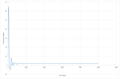
By integration of the velocity autocorrelation function at time $t=0$, the diffusion coefficient can be found.

$D=\frac{1}{3}\underset{0}{\overset{\mathrm{\infty }}{\int }}d\tau ⟨\mathbf{v}(0)\cdot \mathbf{v}(\tau )⟩$

The trapezium rule $\underset{0}{\overset{\mathrm{\infty }}{\int }}f(x)dx=\frac{h}{2}[y_0+y_n+2(y_1+y_2+...+y_{n-2}+y_{n-1})]$ is used to approximate the area under the velocity autocorrelation function for each phase, and the diffusion coefficient determined.

	8,000 molecules	1,000,000 molecules
solid	$8.30\times 10^{-4}$	$4.55\times 10^{-5}$
liquid	$9.79\times 10^{-2}$	$9.01\times 10^{-2}$
vapour	$2.67$	$3.27$

The diffusion coefficients are all of the same magnitude for those calculated using the MSD. Once again the diffusion coefficient of the solid is close to 0 as the system should not undergo Brownian motion so therefore would not be expected have a significant diffusion coefficient. The diffusion coefficient for both methods of determination are very similar, and appears as though 8,000 atoms with 5000 time steps is a large enough simulation to predict the diffusion coefficient to a reasonable degree of accuracy. Although the diffusion coefficient appears to be in agreement with the values from the MSD it can be seen from the VACF that the velocities do not fully decorrelate during the length of the simulations, therefore this value of diffusion coefficient is not reliable.

JC: The velocities do decorrelate for the solid and liquid simulations.

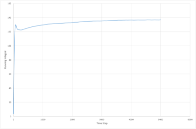
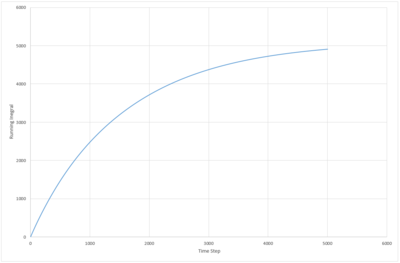
The running integral of the VACF plot for both the 8,000 and 1,000,000 molecule systems were plotted. The biggest source of error in the diffusion coefficients calculated from the VACF is probably due to the false assumption that the systems have reached equilibrium. The system with 8000 atoms must take longer to reach a stable state as the lower density means less collisions occur in the same period of time.

JC: What about the error from using the trapezium rule?

Figure (14). Plots of Running Integral of VACF for three different phases.

	8,000 molecules	1,000,000 molecules
solid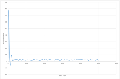
liquid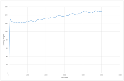
vapour

Conclusion

Simple simulations of Lennard-Jones fluids were run under a variety of different conditions. An optimum time step was determined by plotting energy timestep graphs for different values of timestep. 0.0025 was found to be optimum, as it gave a accurate values, whilst also allowing the simulation to run for long enough that the system could equilibrate correctly. Plots of the simulated density against temperature where compared to the density given by the ideal gas law, and the differences between them were due to repulsive forces felt in the Lennard Jones potential at small values of the internuclear range.

A script was then written to return values for the heat capacity over a range of densities and temperatures. It was seen that the heat capacity does not increase with temperature, which is what would be classically predicted. Instead two regimes inside the simulations cause a lowering of the heat capacity across the transition.

The structure of a Lennard-Jones fluid was observed using the Radial Distriubtion function. The lattice spacing was found to be between 1.45 and 1.48, in reduced units. The number of nearest neighbors were determined using the running integral of the solid RDF.

Simulations of more atoms were found to be more stable, when considering the mean squared displacement and the velocity autocorrelation function and the diffusion coefficient was determined using the two different graphs. The values of the diffusion coefficient returned were relatively similar across the two methods, especially for the liquid and vapour phases although as the gas never appeared to reach an equilibrium value in the VACF it may not be a reliable method of determination. The diffusion coefficients determined from the VACF were all slightly higher than those determined by the MSD. In literature it has been reported than simulations with 100,000 time steps can accurately detemine the diffusion coefficient.

References

- ↑ Bolmatov D., Brazhkin V.V., Trachenko K., Thermodynamic behavious of supercritical matter, Nature Communications [Online] 2013 4 (2331) Available from: doi:10.1038/ncomms3331
- ↑ 2.0 2.1 Hansen J-P., Verlet Loup, Phase Transitions of the Lennard-Jones System Physical Review 1969 184(1) 155 Acessible at: http://journals.aps.org/pr/pdf/10.1103/PhysRev.184.151
- ↑ Schoen M, Hoheisel C, The mutual diffusion coefficient D 12 in binary liquid model mixtures. Molecular dynamics calculations based on Lennard-Jones (12-6) potentials Mol. Phys [Online] 1984 52(1) Available from: DOI:10.1080/00268978400101041 Accessed 26/02/2016