Talk:Mod:ld2113

JC: General comments: This is an excellent report. You demonstrate a very good understanding of the tasks and the background material and give very clear, concise explanations, well done.

Third Year Liquid Simulation Experiment

Introduction to molecular dynamics simulation

Numerical integration

TASK: Open the file HO.xls. In it, the velocity-Verlet algorithm is used to model the behaviour of a classical harmonic oscillator. Complete the three columns "ANALYTICAL", "ERROR", and "ENERGY": "ANALYTICAL" should contain the value of the classical solution for the position at time $t$, "ERROR" should contain the absolute difference between "ANALYTICAL" and the velocity-Verlet solution (i.e. ERROR should always be positive -- make sure you leave the half step rows blank!), and "ENERGY" should contain the total energy of the oscillator for the velocity-Verlet solution. Remember that the position of a classical harmonic oscillator is given by $x\left(t\right)=A\cos (\omega t+\varphi )$ (the values of $A$, $\omega$, and $\varphi$ are worked out for you in the sheet).

The position of the classical harmonic oscillator as a function of time was determined using $x\left(t\right)=A\cos (\omega t+\varphi )$ with $A=1.0$, $\omega =1.0$, and $\varphi =0.0$

Figure 1:Position of a classical harmonic oscillator as a function of time (timestep=0.1)

From figure 1 it can be seen that the results from the Velocity-Verlet algorithm (blue dots) agree very well with the classical solution for the position (red line).

The energy of the classical harmonic oscillator was determined using $E=\frac{1}{2}m{v}^2+\frac{1}{2}k{x}^2$ with $m=1.0$, $k=1.0$ and $x\left(t\right)$ as determined above.

Figure 2:Energy of a classical harmonic oscillator as a function of time (timestep=0.1)

For the energy as a function of position, the results from the simulation (figure 2) differ from what would be expected for an ideal harmonic oscillator. While in figure 2 the total energy is fluctuating between 0.5000 and 0.4988, it would be expected to be constant for an ideal classical harmonic oscillator (with different contributions of potential and kinetic energy at different positions). The amplitude of the sinusoidal fluctuation is however very small (0.2%) so that the the simulation can be considered to produce acceptable physical behavior.

TASK: For the default timestep value, 0.1, estimate the positions of the maxima in the ERROR column as a function of time. Make a plot showing these values as a function of time, and fit an appropriate function to the data.

Figure 3: Linear fit to the maxima of the error function (showing the discrepancy between the classical solution and the solution from the Velocity-Verlet algorithm)

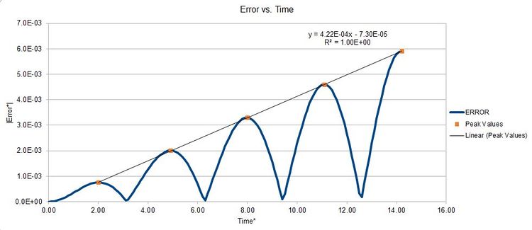
The error function was used to analyse the deviation of the results from the Velocity-Verlet algorithm from the classical solution. Despite no error can be seen upon visible inspection of figure 1, figure 3 shows that there is indeed a small variation between the two solution. The error is biggest for values of $t$ that give $x\left(t\right)$ close to $0$. Furthermore, the error at these points increases linearly with time $(y=4.22*10^{-4}\cdot t+7.30*10^{-5})$. This cumulative increase in the error over time is due to the approximations used in the Velocity-Verlet algorithm, namely the Taylor expansion of the integral.

TASK: Experiment with different values of the timestep. What sort of a timestep do you need to use to ensure that the total energy does not change by more than 1% over the course of your "simulation"? Why do you think it is important to monitor the total energy of a physical system when modelling its behaviour numerically?

Figure 4: Energy oscillation at timestep=0.1

Figure 5: Energy oscillation at timestep=0.2

Figure 6: Energy oscillation at timestep=0.3

It was found that the sinusoidal fluctuation of the energy increases with increasing timesteps while the absolute value of the energy decreases. While for a timestep of 0.1, the fluctuation is very small (figure 4), a timestep of 0.3 produces fluctuations larger than 1% (figure 6). A timestep of 0.2 was found to be the limiting value with fluctuations at 1% (figure 5). Consequently, a timestep below 0.2 has to be chosen ,in order to keep energy fluctuations in the simulations below 1%.

It is important to monitor the total energy of a physical system when modelling its behaviour numerically because only when the system obeys physical laws (energy conservation in this case) to a certain extent, the outputs of the simulation can be considered meaningful.

JC: Good, clear answers to the tasks.

Atomic forces

TASK: For a single Lennard-Jones interaction, $\varphi \left(r\right)=4ϵ(\frac{{\sigma }^{12}}{r^{12}}-\frac{{\sigma }^6}{r^6})$, find the separation, $r_0$, at which the potential energy is zero.

$\varphi \left(r_0\right)=0$

$4ϵ(\frac{{\sigma }^{12}}{r_0^{12}}-\frac{{\sigma }^6}{r_0^6})=0$

$\frac{{\sigma }^{12}}{r_0^{12}}-\frac{{\sigma }^6}{r_0^6}=0$

$\frac{{\sigma }^{12}}{r_0^{12}}=\frac{{\sigma }^6}{r_0^6}$

$\frac{{\sigma }^{12}}{{\sigma }^6}=\frac{r_0^{12}}{r_0^6}$

$r_0=\sigma$

The potential energy is 0 at $r_0=\sigma$.

What is the force at this separation?

For a single particle with

$r=r_0=\sigma$

:

$$\begin{gathered} F=-\frac{\text{d} \\ U\left(r^N\right)}{\text{d} \\ r}=-\frac{\text{d} \\ \varphi \left(r_0\right)}{\text{d} \\ {r}_0}=-\frac{d\left[4ϵ(\frac{{\sigma }^{12}}{r_0^{12}}-\frac{{\sigma }^6}{r_0^6})\right]}{\text{d} \\ {r}_0}=-24ϵ(\frac{{\sigma }^6}{r_0^7}-\frac{2\cdot {\sigma }^{12}}{r_0^{13}})=-24ϵ(\frac{r_0^6}{r_0^7}-\frac{2\cdot r_0^{12}}{r_0^{13}})=\frac{48ϵ}{r_0}-\frac{24ϵ}{r_0}=\frac{24ϵ}{r_0} \end{gathered}$$

At $r=r_0=\sigma$, the force is $F=\frac{24ϵ}{r_0}$.

Find the equilibrium separation, $r_{eq}$, and work out the well depth ($\varphi \left(r_{eq}\right)$).

The system is at equilibrium when

$F=0$

:

$F\left(r_{eq}\right)=0$

$$\begin{gathered} -\frac{\text{d} \\ \varphi \left(r_{eq}\right)}{\text{d} \\ {r}_{eq}}=0 \end{gathered}$$

$$\begin{gathered} -\frac{\text{d}\left[4ϵ(\frac{{\sigma }^{12}}{r_{eq}^{12}}-\frac{{\sigma }^6}{r_{eq}^6})\right]}{\text{d} \\ {r}_{eq}}=0 \end{gathered}$$

$-24ϵ(\frac{{\sigma }^6}{r_{eq}^7}-\frac{2\cdot {\sigma }^{12}}{r_{eq}^{13}})=0$

$\frac{{\sigma }^6}{r_{eq}^7}=2\cdot \frac{{\sigma }^{12}}{r_{eq}^{13}}$

$2{\sigma }^6=r_{eq}^6$

$$\begin{gathered} r_{eq}=\sqrt[6]{2} \\ \sigma \end{gathered}$$

The Equilibrium separation is therefore $$\begin{gathered} r_{eq}=\sqrt[6]{2} \\ \sigma \end{gathered}$$.

Using

$$\begin{gathered} r_{eq}=\sqrt[6]{2} \\ \sigma \end{gathered}$$

:

$$\begin{gathered} \varphi \left(r_{eq}\right)=4ϵ(\frac{{\sigma }^{12}}{{\left(\sqrt[6]{2} \\ \sigma \right)}^{12}}-\frac{{\sigma }^6}{{\left(\sqrt[6]{2} \\ \sigma \right)}^6})=4ϵ(\frac{1}{2^2}-\frac{1}{2})=-ϵ \end{gathered}$$

The well depth at $$\begin{gathered} r_{eq}=\sqrt[6]{2} \\ \sigma \end{gathered}$$ is $\varphi \left(r_{eq}\right)=-ϵ$.

Evaluate the integrals $\underset{2\sigma }{\overset{\mathrm{\infty }}{\int }}\varphi \left(r\right)\mathrm{d}r$, $\underset{2.5\sigma }{\overset{\mathrm{\infty }}{\int }}\varphi \left(r\right)\mathrm{d}r$, and $\underset{3\sigma }{\overset{\mathrm{\infty }}{\int }}\varphi \left(r\right)\mathrm{d}r$ when $\sigma =ϵ=1.0$.

For

$\sigma =ϵ=1.0$

:

$\underset{2\sigma }{\overset{\mathrm{\infty }}{\int }}\varphi \left(r\right)\text{d}r=\underset{2\sigma }{\overset{\mathrm{\infty }}{\int }}4ϵ(\frac{{\sigma }^{12}}{r^{12}}-\frac{{\sigma }^6}{r^6})\text{d}r=\underset{2}{\overset{\mathrm{\infty }}{\int }}4(\frac{1^{12}}{r^{12}}-\frac{1^6}{r^6})\text{d}r=4{(\frac{1}{5r^5}-\frac{1}{11r^{11}})}_2^{\mathrm{\infty }}=-2.48\cdot 10^{-2}$

$\underset{2.5\sigma }{\overset{\mathrm{\infty }}{\int }}\varphi \left(r\right)\text{d}r=4{(\frac{1}{5r^5}-\frac{1}{11r^{11}})}_{2.5}^{\mathrm{\infty }}=-8.18\cdot 10^{-3}$

$\underset{3\sigma }{\overset{\mathrm{\infty }}{\int }}\varphi \left(r\right)\text{d}r=4{(\frac{1}{5r^5}-\frac{1}{11r^{11}})}_3^{\mathrm{\infty }}=-3.29\cdot 10^{-3}$

The solution for the three integrals are therefore:

$\underset{2\sigma }{\overset{\mathrm{\infty }}{\int }}\varphi \left(r\right)\text{d}r=-2.48\cdot 10^{-2}$

$\underset{2.5\sigma }{\overset{\mathrm{\infty }}{\int }}\varphi \left(r\right)\text{d}r=-8.18\cdot 10^{-3}$

$\underset{3\sigma }{\overset{\mathrm{\infty }}{\int }}\varphi \left(r\right)\text{d}r=-3.29\cdot 10^{-3}$

TASK: Estimate the number of water molecules in 1ml of water under standard conditions. Estimate the volume of $10000$ water molecules under standard conditions.

At standard conditions: $$\begin{gathered} \rho =999.8 \\ \frac{kg}{m^3}=0.9998 \\ \frac{g}{mL} \end{gathered}$$, furthermore using $N_A=6.022\cdot 10^{23}\frac{1}{mol}$ and $$\begin{gathered} M_{H_{2}O}=18 \\ \frac{g}{mol} \end{gathered}$$.

$$\begin{gathered} m=\frac{\rho }{V}=\frac{0.9998 \\ \frac{g}{mL}}{1 \\ mL}=0.9998 \\ g \end{gathered}$$

$$\begin{gathered} n=\frac{m}{M}=\frac{0.9998 \\ g}{18 \\ \frac{g}{mol}}=0.05554 \\ mol \end{gathered}$$

$$\begin{gathered} N=n\cdot N_A=0.05554 \\ mol\cdot 6.022\cdot 10^{23}\frac{1}{mol}=3.345\cdot 10^{22} \end{gathered}$$

There hence are approximately $3.345\cdot 10^{22}$ molecules in 1 ml water at standard conditions.

$$\begin{gathered} n=\frac{N}{N_A}=\frac{10,000}{6.022\cdot 10^{23}\frac{1}{mol}}=1.661\cdot 10^{-20} \\ mol \end{gathered}$$

$$\begin{gathered} m=M\cdot n=18 \\ \frac{g}{mol}\cdot 1.661\cdot 10^{-20} \\ mol=2.990\cdot 10^{-19} \\ g \end{gathered}$$

$$\begin{gathered} V=\frac{m}{\rho }=\frac{2.9898\cdot 10^{-19} \\ g}{0.9998 \\ \frac{g}{mL}}=2.9904\cdot 10^{-19} \\ ml=299.04 \\ n{m}^3 \end{gathered}$$

At standard conditions, 10,000 water molecules populate approximately $$\begin{gathered} 2.9904\cdot 10^{-19} \\ ml \end{gathered}$$ or $$\begin{gathered} 299.04 \\ n{m}^3 \end{gathered}$$ of space.

JC: All maths correct and very clearly laid out.

TASK: Consider an atom at position $(0.5,0.5,0.5)$ in a cubic simulation box which runs from $(0,0,0)$ to $(1,1,1)$. In a single timestep, it moves along the vector $(0.7,0.6,0.2)$. At what point does it end up, after the periodic boundary conditions have been applied?.

Without periodic boundary conditions, the atom would be outside the box after one timestep. Namely in position $(1.2,1.1,0.7)$. With the applied periodic boundary conditions, the atom would be in position $(0.2,0.1,0.7)$ inside the box.

JC: Correct.

TASK: The Lennard-Jones parameters for argon are $$\begin{gathered} \sigma =0.34\mathrm{n}\mathrm{m},ϵ \\ / \\ {k}_B=120\mathrm{K} \end{gathered}$$. If the LJ cutoff is $r^{*}=3.2$, what is it in real units? What is the well depth in $$\begin{gathered} {\mathrm{k}\mathrm{J} \\ \mathrm{m}\mathrm{o}\mathrm{l}}^{-1} \end{gathered}$$? What is the reduced temperature $T^{*}=1.5$ in real units?

$$\begin{gathered} r=r^{*}\cdot \sigma =3.2\cdot 0.34 \\ nm=1.1 \\ nm \end{gathered}$$

$$\begin{gathered} {ϵ}_m=ϵ\cdot N_A=120 \\ \text{K}\cdot k_B\cdot N_A=120 \\ \text{K}\cdot 1.381\cdot 10^{-26} \\ \frac{kJ}{K}\cdot 6.022\cdot 10^{23}\frac{1}{mol}=0.997 \\ \frac{kJ}{mol} \end{gathered}$$

$$\begin{gathered} T=\frac{T^{*}\cdot ϵ}{k_B}=1.5\cdot 120 \\ \text{K}=180\text{K} \end{gathered}$$

In real units, the LJ cutoff is $$\begin{gathered} r=1.1 \\ nm \end{gathered}$$, the well depth is $$\begin{gathered} {ϵ}_m=0.997 \\ \frac{kJ}{mol} \end{gathered}$$ and the Temperature is $T=180\text{K}$.

JC: Correct.

Equilibration

Creating the simulation box

TASK: Why do you think giving atoms random starting coordinates causes problems in simulations? Hint: what happens if two atoms happen to be generated close together?

Due to the high number of atoms "placed" in the box, there would be a high probability of certain atoms being placed significantly closer together than their equilibrium distance when assigning random starting coordinates to the atoms. In such an event, the atom pair interaction(Lennard-Jones potential) for that specific would be extremely high. Such high potentials would lead to a simulated system that is not a good representation of reality and hence giving inaccurate results when measuring the properties of the system.

JC: A system with very high repulsion forces between atoms will be unstable, which often causes the simulation to crash.

TASK: Satisfy yourself that this lattice spacing $(1.07722)$ corresponds to a number density of lattice points of $0.8$. Consider instead a face-centred cubic lattice with a lattice point number density of 1.2. What is the side length of the cubic unit cell?

The number density is defined as $\rho =\frac{n}{V}$ and the volume can be calculated from the lattice spacing $x$: $V=x^3$. As it can be seen from figure 6, there is 1 lattice point per unit cell $(4\cdot \frac{1}{4}=1)$. The number density in a simple cubic lattice with side length $x=1.07722$ is therefore: $\rho =\frac{n}{x^3}=\frac{1}{1.07722^3}=\frac{1}{1.25}=0.8$ ---- In a fcc lattice (figure 7) there are 4 lattice points per unit cell $(6\cdot \frac{1}{2}+8\cdot \frac{1}{8}=4)$. Rearranging the formular above to $x=\sqrt[3]{\frac{n}{\rho }}$ with $\rho =1.2$ gives: $x=\sqrt[3]{\frac{4}{1.2}}=1.49$ The side length of a fcc lattice with number density $\rho =1.2$ is therefore $x=1.49$.

File:Lattic simple cubic.svg Fig. 6: Simple cubic lattice with lattice spacing a File:Lattice face centered cubic.svg Fig. 7: Face centered cubic lattice with lattice spacing a

TASK: Consider again the face-centred cubic lattice from the previous task. How many atoms would be created by the create_atoms command if you had defined that lattice instead?

region box block 0 10 0 10 0 10
create_box 1 box
create_atoms 1 box

Given that there are 4 lattice points per unit cell $(6\cdot \frac{1}{2}+8\cdot \frac{1}{8}=4)$ in a fcc lattice, this command would have created $4\cdot 10\cdot 10\cdot 10=4000$ atoms.

JC: Correct.

Setting the properties of the atoms

TASK: Using the LAMMPS manual, find the purpose of the following commands in the input script:

mass 1 1.0
pair_style lj/cut 3.0
pair_coeff * * 1.0 1.0

mass 1 1.0 sets the mass of all atoms of type '1' to 1.0.
pair_style lj/cut 3.0 defines the interaction between atom pairs in the simulation. In this case, a Lennard-Jones potential will be used , but only up to a cut off distance of 3.0 (red. units). As the Lennard-Jones potential decreases rapidly with increasing distance, this is a good approximation to make. Without defining a cutoff distance, an infinite number of atomic interactions would have to be computed, given the periodic boundary conditions we are using in this simulation.
pair_coeff * * 1.0 1.0 defines the pairwise force field coefficients for all atom types (*) in the simulation. In this case the coefficients are both 1.0.

TASK: Given that we are specifying ${\mathbf{x}}_i\left(0\right)$ and ${\mathbf{v}}_i\left(0\right)$, which integration algorithm are we going to use?

We are using the Velocity-Verlet integration mechanism, as it requires the position and velocity at time 0 as a starting point (i.e. ${\mathbf{x}}_i\left(0\right)$ and ${\mathbf{v}}_i\left(0\right)$).

Running the simulation

TASK: Look at the lines below.

### SPECIFY TIMESTEP ###
variable timestep equal 0.001
variable n_steps equal floor(100/${timestep})
variable n_steps equal floor(100/0.001)
timestep ${timestep}
timestep 0.001

### RUN SIMULATION ###
run ${n_steps}
run 100000

The second line (starting "variable timestep...") tells LAMMPS that if it encounters the text ${timestep} on a subsequent line, it should replace it by the value given. In this case, the value ${timestep} is always replaced by 0.001. In light of this, what do you think the purpose of these lines is? Why not just write:

timestep 0.001
run 100000

Defining a timestep and a n_steps variable and then linking the two as done above means that only the timestep will have to be changed when altering the conditions of the simulation. The number of steps will change accordingly so that total simulated time will always be constant. This ensures the production of comparable results when altering simulation conditions.

JC: Good explanation.

Checking equilibration

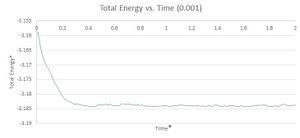
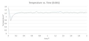
TASK: make plots of the energy, temperature, and pressure, against time for the 0.001 timestep experiment (attach a picture to your report). Does the simulation reach equilibrium? How long does this take? When you have done this, make a single plot which shows the energy versus time for all of the timesteps (again, attach a picture to your report). Choosing a timestep is a balancing act: the shorter the timestep, the more accurately the results of your simulation will reflect the physical reality; short timesteps, however, mean that the same number of simulation steps cover a shorter amount of actual time, and this is very unhelpful if the process you want to study requires observation over a long time. Of the five timesteps that you used, which is the largest to give acceptable results? Which one of the five is a particularly bad choice? Why?

Figure 8: Total energy vs time for timestep=0.001	Figure 9: Temperature vs time for timestep=0.001	Figure 10: Pressure vs time for timestep=0.001	Figure 11: Total energy vs time for all computed timesteps
Figure 12: Zoom: Total energy vs time for timestep=0.001	Figure 13: Zoom: Temperature vs time for timestep=0.001	Figure 14: Zoom: Pressure vs time for timestep=0.001	Figure 15: Zoom: Total energy vs time for all computed timesteps

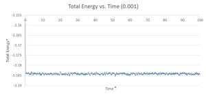
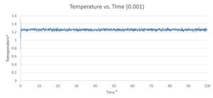
From inspection of figures (8 - 10), it can be seen that equilibrium (i.e. relatively constant temperature, pressure and total energy) is reached. Figures 12 - 114 show that this occurs at approximately $t^{*}=0.3$. The average total energy, temperature and pressure after reaching equilibrium is $E^{*}=-3.18$, $T^{*}=1.26$ and $P^{*}=2.62$ respectively.

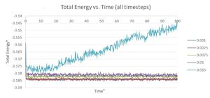
As timestep=0.0025 gives roughly the same results for the total energy as timestep=0.001 and all larger timesteps produce substantial deviation from it, timestep=0.0025 can be considered the largest one to give acceptable results. Using timestep=0.0025 instead of timestep=0.001, longer time frames can be simulated without negatively affecting the results.

For timestep=0.0075 and timestep=0.01 it was found (figure 11) that the total energy of the system increases for larger timesteps but still reaches equilibrium (however, with larger fluctuations around the average value with increasing timestep). For timestep=0.015 however, equilibrium was not reached for $t^{*}>20$ as can be seen from the same figure. Timestep=0.015 therefore is a particularly bad choice, as the lack of equilibrium will avoid any meaningful results to be found from the simulation.

JC: Good choice of timestep and clear justification.

Running simulations under specific conditions

TASK: Choose 5 temperatures (above the critical temperature $T^{*}=1.5$), and two pressures (you can get a good idea of what a reasonable pressure is in Lennard-Jones units by looking at the average pressure of your simulations from the last section). This gives ten phase points — five temperatures at each pressure. Create 10 copies of npt.in, and modify each to run a simulation at one of your chosen $(p,T)$ points. You should be able to use the results of the previous section to choose a timestep. Submit these ten jobs to the HPC portal. While you wait for them to finish, you should read the next section.

Based on the findings from the previous section, $timestep=0.0025$ and $P^{*}=2.4$ and $P^{*}=2.6$ was used for these simulations. $T^{*}$ was chosen as $1.5,2.0,3.0,4.0,5.0$.

Thermostats and Barostats

TASK: We need to choose $\gamma$ so that the temperature is correct $T=\mathfrak{𝔗}$ if we multiply every velocity $\gamma$. We can write two equations:

$\frac{1}{2}\sum _i{m}_i{v}_i^2=\frac{3}{2}N{k}_{B}T$

$\frac{1}{2}\sum _i{m}_i{\left(\gamma v_i\right)}^2=\frac{3}{2}N{k}_B\mathfrak{𝔗}$

Solve these to determine $\gamma$.

Multiplying the velocity with $\gamma$ ensures that the fluctuations of $\mathfrak{𝔗}$ around the set value $T$ are compensated for at every timestep. To derive an expression for $\gamma$, the two equations above can be added together to give:

$\frac{1}{2}\sum _i{m}_i{v}_i^2+\frac{1}{2}\sum _i{m}_i{\left(\gamma v_i\right)}^2=\frac{3}{2}N{k}_{B}T+\frac{3}{2}N{k}_B\mathfrak{𝔗}$

Moving the constant $\gamma$ out of the summed term, allows to rearrange the equation to:

$(1+{\gamma }^2)\frac{1}{2}\sum _i{m}_i{v}_i^2=(T+\mathfrak{𝔗})\frac{3}{2}N{k}_B$

$(1+{\gamma }^2)\sum _i{m}_i{v}_i^2=(T+\mathfrak{𝔗})3N{k}_B$

Using $\frac{1}{2}\sum _i{m}_i{v}_i^2=\frac{3}{2}N{k}_{B}T$ from above, we can now write:

$(1+{\gamma }^2)3N{k}_{B}T=(T+\mathfrak{𝔗})3N{k}_B$

$(1+{\gamma }^2)T=(T+\mathfrak{𝔗})$

${\gamma }^2=\left(\frac{T+\mathfrak{𝔗}}{T}\right)-1$

${\gamma }^2=1+\left(\frac{\mathfrak{𝔗}}{T}\right)-1$

${\gamma }^2=\frac{\mathfrak{𝔗}}{T}$

$\gamma =\sqrt{\frac{\mathfrak{𝔗}}{T}}$

The expression for$\gamma$ is therefore $\gamma =\sqrt{\frac{\mathfrak{𝔗}}{T}}$.

JC: Good derivation.

Examining the Input Script

TASK: Use the manual page to find out the importance of the three numbers 100 1000 100000. How often will values of the temperature, etc., be sampled for the average? How many measurements contribute to the average? Looking to the following line, how much time will you simulate?

fix aves all ave/time 100 1000 100000 v_dens v_temp v_press v_dens2 v_temp2 v_press2
run 100000

The first number declares that every 100th timestep should be sampled to calculate the average. The second number declares that this should be carried out 1000 times, so that the average will cover 10,000 timesteps (the third number). For our simulation of 10,000 atoms, we will therefore be calculating 1 average value to which every 100th timestep contributes.

The following line states, that 100000 calculations should be run. With a timestep of 0.0025, this corresponds to a time of 250 reduced time units.

Plotting the Equations of State

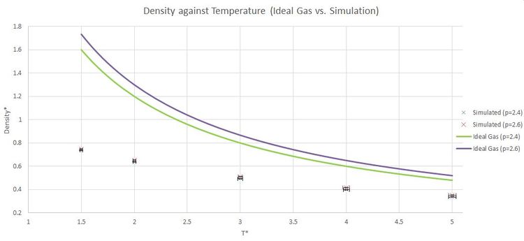
TASK: When your simulations have finished, download the log files as before. At the end of the log file, LAMMPS will output the values and errors for the pressure, temperature, and density $\left(\frac{N}{V}\right)$. Use software of your choice to plot the density as a function of temperature for both of the pressures that you simulated. Your graph(s) should include error bars in both the x and y directions. You should also include a line corresponding to the density predicted by the ideal gas law at that pressure. Is your simulated density lower or higher? Justify this. Does the discrepancy increase or decrease with pressure?

From figure 16, it can be seen that he simulated density is lower than the density of an ideal gas at the given temperatures and pressures. This can be explained by comparing the approximations with regards to particle interaction (i.e. potential energy) made in the simulation and an ideal gas. With the absence of particle interaction as assumed in the ideal gas, particles can move very closely to each other without increasing potential energy. In the simulation however, the repulsive term of the Lennard-Jones potential causes an increased potential energy (i.e. unfavourable interaction) between particles that are very close together. It is therefore favourable for the particles in the simulation not to be closer to each other than a minimum distance. This Property causes the average density of the simulated system to be lower that in an ideal gas.

It can also be seen, that for higher pressures (as well as lower temperatures) the discrepancy in higher. This can be can be explained by the fact that at low pressures as well as at high temperatures, the systems behave similar to an ideal gas with little interaction between particles. For high pressures and low temperatures however, particles move slower, are closer together in space and therefore interact more. This makes the system increasingly different to the ideal gas with increasing pressure and decreasing temperature where no particle interaction (i.e. potential energy) is assumed.

Fig. 16: Density as a function of temperature from simulation and for ideal gas

JC: Well explained.

Calculating heat capacities using statistical physics

TASK: As in the last section, you need to run simulations at ten phase points. In this section, we will be in density-temperature $({\rho }^{*},T^{*})$ phase space, rather than pressure-temperature phase space. The two densities required at $0.2$ and $0.8$, and the temperature range is $2.0,2.2,2.4,2.6,2.8$. Plot $C_V/V$ as a function of temperature, where $V$ is the volume of the simulation cell, for both of your densities (on the same graph). Is the trend the one you would expect? Attach an example of one of your input scripts to your report.

From figure 17 it can be seen that heat capacity per volume increases with density. As heat capacity is an extensive property, it is expected to increase with the number of atoms present. The heat capacity per volume is therefore expected to increase with the number of atoms per unit volume. As number density is defined as the number of atoms per unit volume, it is expected that the heat capacity per unit volume increases with density.

It can also be seen from the same figure that heat capacity per unit volume decreases with temperature. This observation is not very straight forward to explain and a thorough explanation would require a detailed inspection of the electronic structure of the material. Heat capacity is defined as the energy required per increase in unit temperature, i.e. the energy required to bring the system to a higher energy state. Based on the general assumption that energy levels are more closely spaced with increasing energy (i.e. increasing temperature) it only is a logical consequence that the heat capacity per unit volume decreases with increasing temperature.

JC: Good explanation of both trends. Further analysis without electronic structure calculations would be needed to give a more detailed explanation of the change in heat capacity with temperature for the classical Lennard Jones system that you are simulating here.

Fig. 17: Heat capacity per volume as a function of temperature for different densities

The following script was used for the simulation at phase point $$\begin{gathered} {\rho }^{*}=0.2 \\ {T}^{*}=2.0 \end{gathered}$$:

### DEFINE SIMULATION BOX GEOMETRY ###
variable d equal 0.2
lattice sc ${d}
region box block 0 15 0 15 0 15
create_box 1 box
create_atoms 1 box

### DEFINE PHYSICAL PROPERTIES OF ATOMS ###
mass 1 1.0
pair_style lj/cut/opt 3.0
pair_coeff 1 1 1.0 1.0
neighbor 2.0 bin

### SPECIFY THE REQUIRED THERMODYNAMIC STATE ###
variable T equal 2.0
variable timestep equal 0.0025

### ASSIGN ATOMIC VELOCITIES ###
velocity all create ${T} 12345 dist gaussian rot yes mom yes

### SPECIFY ENSEMBLE ###
timestep ${timestep}
fix nve all nve

### THERMODYNAMIC OUTPUT CONTROL ###
thermo_style custom time etotal temp press
thermo 10

### RECORD TRAJECTORY ###
dump traj all custom 1000 output-1 id x y z

### SPECIFY TIMESTEP ###

### RUN SIMULATION TO MELT CRYSTAL ###
run 10000
unfix nve
reset_timestep 0

### BRING SYSTEM TO REQUIRED STATE ###
variable tdamp equal ${timestep}*100
variable pdamp equal ${timestep}*1000
fix nvt all nvt temp ${T} ${T} ${tdamp}
run 10000
reset_timestep 0
unfix nvt
fix nve all nve

### MEASURE SYSTEM STATE ###
thermo_style custom step etotal temp
variable temp equal temp
variable etotal equal etotal
variable etotal2 equal etotal*etotal
fix aves all ave/time 100 1000 100000 v_temp v_etotal v_etotal2
run 100000

variable avetemp equal f_aves[1]
variable avetemp2 equal f_aves[1]*f_aves[1]
variable aveetotal equal f_aves[2]
variable aveetotal2 equal f_aves[3]
variable ave2etotal equal f_aves[2]*f_aves[2]
variable volume equal vol
variable n equal atoms
variable n2 equal atoms*atoms
variable cv equal ((${n2}*(${aveetotal2}-${ave2etotal}))/(${avetemp2}))
variable cvv equal (${cv}/${volume})

print "Averages"
print "--------"
print "Density: ${d}"
print "AveTemperature: ${avetemp}"
print "Volume: ${volume}"
print "HeatCapacity: ${cv}"
print "HeatCapacityPerVolume: ${cvv}"

Structural properties and the radial distribution function

TASK: perform simulations of the Lennard-Jones system in the three phases. When each is complete, download the trajectory and calculate $g(r)$ and $\int g(r)\mathrm{d}r$. Plot the RDFs for the three systems on the same axes, and attach a copy to your report. Discuss qualitatively the differences between the three RDFs, and what this tells you about the structure of the system in each phase. In the solid case, illustrate which lattice sites the first three peaks correspond to. What is the lattice spacing? What is the coordination number for each of the first three peaks?

Looking at a phase diagram for the Lennard-Jones system, the values were chosen as follows. Liquid:$$\begin{gathered} {\rho }^{*}=0.8 \\ {T}^{*}=1.2 \end{gathered}$$ Solid:$$\begin{gathered} {\rho }^{*}=1.2 \\ {T}^{*}=1.2 \end{gathered}$$ Vapour:$$\begin{gathered} {\rho }^{*}=0.05 \\ {T}^{*}=1.2 \end{gathered}$$

Figure 18: Radial distribution function for vapour, liquid, solid and gas

Figure 19: Running integral for the radial distribution function

Figure 20: Fcc lattice with three nearest coordination sites of central atom (red) highlighted (taken and amended from Wikimedia)

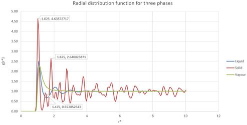
Looking at figure 18, it can be seen that while all three phases have a very different RDFs,it is the same for all three of them up to ca. $r^{*}=0.9$. As the RDF represents the atom density around any molecule in the system, the RDF being 0 up to that distance indicates that no neighbouring atoms can be found in that region around the atom. This can be explained by considering the Lennard-Jones potential which was used to simulate the interatomic interactions in this system: for small values of $r^{*}$, the potential energy becomes vary hight, making a configuration with $r^{*}<0.9$ very energetically unfavourable.

The RDF of the gas shows a single broad peak at $r^{*}=1.125$ and then shows a smooth straight line. This behaviour of the curve is produced by the very low degree of order in a gas which averages the atomic density around an atom to a straight line.

The RDF of the liquid shows three broad peaks of decreasing intensity before becoming a straight line. This indicates an increased degree of order close to the atom in a liquid compared to gas. Due to the atoms still being able to move relatively freely in a liquid, no long-range order can be achieved so that the RDF averages out to a straight line for large values of $r^{*}$.

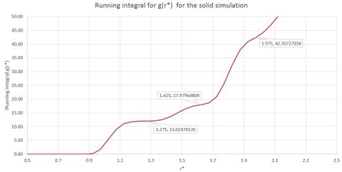
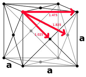
For the solid, the RDF is showing sharp peaks over the whole analysed distance range this indicates a high degree of order (both short and long range) with atoms repeatedly being in the same locations in all direction from the inspected atom. In this system the atoms can be considered fixed in their position of the fcc lattice so that the peaks of the RDF can be assigned to specific coordination sites in the lattice. Figure 20 shows the lattice sites that the first three peaks correspond to. From this figure, it can be seen that the lattice spacing is approximately 1.475 reduced units.

From the integral of the radial distribution function (figure 19) as well as figure 20, the coordination number for the first three peaks can be determined as 12,6 and 24 respectively.

JC: Good understanding of the RDFs for the different phases. Can you show that the positions (r) of the first three peaks in the solid RDF corresponds to the distances to the first, second and third nearest neighbours in the fcc structure?/span>

Dynamical properties and the diffusion coefficient

TASK: In the D subfolder, there is a file liq.in that will run a simulation at specified density and temperature to calculate the mean squared displacement and velocity autocorrelation function of your system. Run one of these simulations for a vapour, liquid, and solid. You have also been given some simulated data from much larger systems (approximately one million atoms). You will need these files later.

Simulations in this Section

TASK: make a plot for each of your simulations (solid, liquid, and gas), showing the mean squared displacement (the "total" MSD) as a function of timestep. Are these as you would expect? Estimate $D$ in each case. Be careful with the units! Repeat this procedure for the MSD data that you were given from the one million atom simulations.

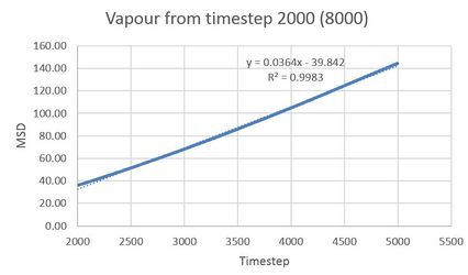
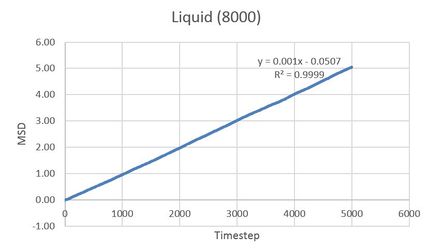
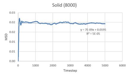
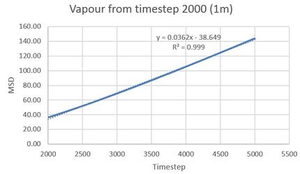
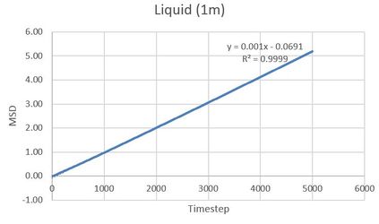
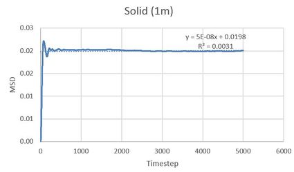
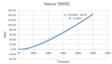
The diffusion coefficient can be determined using $D=\frac{1}{6}\frac{\partial ⟨r^2\left(t\right)⟩}{\partial t}$. The gradient of the MSD $\frac{\partial ⟨r^2\left(t\right)⟩}{\partial t}$ can be found from the plots below. As the data in the plots is in timestep units, the gradient has to be multiplied by 0.002 to make sure the units match up.

Figure 21: MSD for 8000 atoms in vapour phase

Figure 22: MSD for 1m atoms in vapour phase

For the gas phase (figure 21 and 22), linear behaviour is only observed after 2000 timesteps. Before that the behaviour resembles a quadratic function. This can be explained by the atoms not colliding regularly at the beginning of the simulation but rather moving through space freely (as they are too far apart). Their displacement therefore increases linearly with time and their mean squared displacement increases squared with time.

As we are only interested in the properties of the system once it has reached a stable state and atoms collide, the gradients for the gas were determined using only timestep values greater than 2000 (figure 23 and 26).

JC: Good reasoning, no need to show a linear fit to all the data in figure 21, this is slightly confusing.

From 2000 timestep onwards for the vapour and from 0 timestep onwards for the liquid, a linear relationship between the MSD and timestep is observed (see figure 23, 24, 26 and 27). This resembles the expected behaviour of the atoms moving and colliding randomly. This behaviour is known as brownian motion. It can also be seen from the same figures that the diffusion coefficients are much higher for the gas compared to the liquid, this agrees with the idea that atoms in the gas phase can move more freely than in atoms in the liquid phase.

The diffusion coefficients for the solid are the lowest of the three phases and does not increase linearly with timestep. It rather increases rapidly and then stays more or less constant for the duration of the simulation. This agrees with the notion that atoms in a solid cannot move freely once they have reached the position of lowest potential with regards to their neighbours.

The difference between the 8000 and the 1m atom simulations (and the respective diffusion coefficients) are generally very low. This suggests that the 8000 atom simulation resembles a real physical system reasonably well.

Figure 23: MSD for 8000 atoms in vapour phase (timestep from 2000)	Figure 24: MSD for 8000 atoms in liquid phase	Figure 25: MSD for 8000 atoms in solid phase
Diffusion coefficient vapour: $D=3.03$	Diffusion coefficient liquid: $D=8.33\cdot 10^{-2}$	Diffusion coefficient solid: $D=5.83\cdot 10^{-7}$

Figure 26: MSD for 1m atoms in vapour phase (timestep from 2000)	Figure 27: MSD for 1m atoms in liquid phase	Figure 28: MSD for 1m atoms in solid phase
Diffusion coefficient vapour (1m): $D=3.02$	Diffusion coefficient liquid (1m): $D=8.33\cdot 10^{-2}$	Diffusion coefficient solid (1m): $D=4.17\cdot 10^{-6}$

Velocity Autocorrelation Function

TASK: In the theoretical section at the beginning, the equation for the evolution of the position of a 1D harmonic oscillator as a function of time was given. Using this, evaluate the normalised velocity autocorrelation function for a 1D harmonic oscillator (it is analytic!):

$C\left(\tau \right)=\frac{\underset{-\mathrm{\infty }}{\overset{\mathrm{\infty }}{\int }}v\left(t\right)v(t+\tau )\mathrm{d}t}{\underset{-\mathrm{\infty }}{\overset{\mathrm{\infty }}{\int }}{v}^2\left(t\right)\mathrm{d}t}$

Be sure to show your working in your writeup.

Stating from the equation of the position of the harmonic oscillator:

$x\left(t\right)=A\cos (\omega t+\varphi )$

We get the velocity by taking the derivative:

$v\left(t\right)=\frac{\text{d}x\left(t\right)}{\text{d}t}=-A\omega \sin (\omega t+\varphi )$

$v(t+\tau )=-A\omega \sin (\omega (t+\tau )+\varphi )$

Substituting into original equation:

$$\begin{gathered} C(\tau )=\frac{\underset{-\mathrm{\infty }}{\overset{\mathrm{\infty }}{\int }}(-A\omega \sin (\omega t+\varphi ))\cdot (-A\omega \sin (\omega (t+\tau )+\varphi )\text{d}t}{\underset{-\mathrm{\infty }}{\overset{\mathrm{\infty }}{\int }}(A^2{\omega }^2 \\ si{n}^2(\omega t+\varphi ))\text{d}t}=\frac{\underset{-\mathrm{\infty }}{\overset{\mathrm{\infty }}{\int }}(-A\omega \sin (\omega t+\varphi ))\cdot (-A\omega \sin (\omega (t+\tau )+\varphi )\text{d}t}{\underset{-\mathrm{\infty }}{\overset{\mathrm{\infty }}{\int }}{\sin }^2(\omega t+\varphi )\text{d}t} \end{gathered}$$

Using the trigonometric identity $sin(a+b)=sin(a)cos(b)+sin(b)cos(a)$ we can write:

$C(\tau )=\frac{\underset{-\mathrm{\infty }}{\overset{\mathrm{\infty }}{\int }}(sin(\omega t+\varphi ))[sin(\omega t+\varphi )cos(\omega \tau )+cos(\omega t+\varphi )sin(\omega \tau )]\text{d}t}{\underset{-\mathrm{\infty }}{\overset{\mathrm{\infty }}{\int }}si{n}^2(\omega t+\varphi )\text{d}t}=\frac{\underset{-\mathrm{\infty }}{\overset{\mathrm{\infty }}{\int }}si{n}^2(\omega t+\varphi )cos(\omega \tau )+sin(\omega t+\varphi )cos(\omega t+\varphi )sin(\omega \tau )\text{d}t}{\underset{-\mathrm{\infty }}{\overset{\mathrm{\infty }}{\int }}si{n}^2(\omega t+\varphi )\text{d}t}$

$=\frac{cos(\omega \tau )\underset{-\mathrm{\infty }}{\overset{\mathrm{\infty }}{\int }}si{n}^2(\omega t+\varphi )\text{d}t+sin(\omega \tau )\underset{-\mathrm{\infty }}{\overset{\mathrm{\infty }}{\int }}sin(\omega t+\varphi )cos(\omega t+\varphi )\text{d}t}{\underset{-\mathrm{\infty }}{\overset{\mathrm{\infty }}{\int }}si{n}^2(\omega t+\varphi )\text{d}t}=cos(\omega \tau )+\frac{sin(\omega \tau )\underset{-\mathrm{\infty }}{\overset{\mathrm{\infty }}{\int }}sin(\omega t+\varphi )cos(\omega t+\varphi )\text{d}t}{\underset{-\mathrm{\infty }}{\overset{\mathrm{\infty }}{\int }}si{n}^2(\omega t+\varphi )\text{d}t}$

The second term

$\underset{-\mathrm{\infty }}{\overset{\mathrm{\infty }}{\int }}sin(\omega t+\varphi )cos(\omega t+\varphi )\text{d}t$

is zero as we're integrating an antisymmetric function from

$-\mathrm{\infty }$

to

$\mathrm{\infty }$

. Hence:

$C(\tau )=cos(\omega \tau )$

JC: Good, clear derivation.

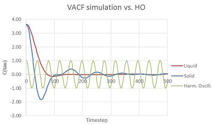
On the same graph, with x range 0 to 500, plot $C\left(\tau \right)$ with $\omega =1/2\pi$ and the VACFs from your liquid and solid simulations. What do the minima in the VACFs for the liquid and solid system represent? Discuss the origin of the differences between the liquid and solid VACFs. The harmonic oscillator VACF is very different to the Lennard Jones solid and liquid. Why is this? Attach a copy of your plot to your writeup.

From the radial distribution function of the liquid and solid in the previous section, we can see how the surroundings of an atom is different for the two systems. While in the solid the atoms are in a fixed lattice around the inspected atom (short range and long range order), in the liquid only short range order is observed. The comparatively stronger minima in the solid therefore correspond to the large change in velocity upon collision with neighbouring atoms whereas the comparatively weak initial minimum in the liquid corresponds to collision only with the ordered atoms in close proximity of the inspected atom (cf. solvation shell).

For both the liquid and the solid the VACF goes to zero over time. This is because due to repeating collisions the velocity of the atoms becomes decorrelated over time. The model of an harmonic oscillator does not account for any collisions so that the velocity does not get decorrelated over time. It therefore makes sense that the VACF does not go to zero over time; it rather oscillates around 0. The VACF of the harmonic oscillator is zero at maximum and minimum atom distance as the velocity is constant at that point in time.

Figure 29: $C\left(\tau \right)$ for simulation of solid, liquid anda harmonic oscillator

TASK: Use the trapezium rule to approximate the integral under the velocity autocorrelation function for the solid, liquid, and gas, and use these values to estimate $D$ in each case. You should make a plot of the running integral in each case. Are they as you expect? Repeat this procedure for the VACF data that you were given from the one million atom simulations. What do you think is the largest source of error in your estimates of D from the VACF?

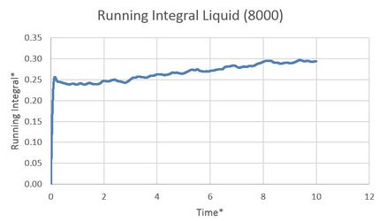
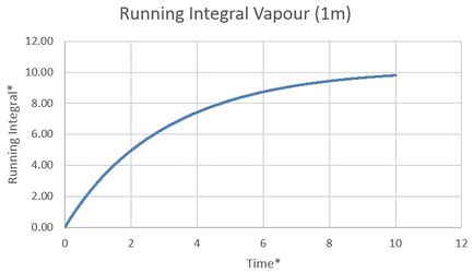
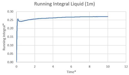
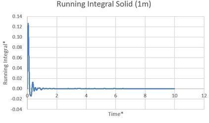
The diffusion coefficients were determined from the running integrals of the VACF after converting the timestep into time* to ensure consistent units. The formula given was $D=\frac{1}{3}\underset{0}{\overset{\mathrm{\infty }}{\int }}\mathrm{d}\tau ⟨\mathbf{v}\left(0\right)\cdot \mathbf{v}\left(\tau \right)⟩$.

As expected, the diffusion coefficients found from integrating the VACF are smallest for the solid, and largest for the gas. The diffusion coefficients are also reasonably similar to the ones found from the MSD above. This suggests that they both reasonable ways to calculate the diffusion coefficient.

Besides the inherent inherent error in any numerical integration method, the VACF would have to be integrated to infinity as stated in the formula above. As this is not possible for our simulation (it would require infinite computation time), the calculated diffusion coefficient will not be completely accurate. As the VACF tends to zero for our simulated system for large time, this value is however not extraordinarily high. When comparing figure 31 and 34 it can also be seen that noise in the VACF decreases with increasing number of particles. Noise can therefore also be a significant source of error when simulating small systems.

Figure 30: Running integral for VACF of 8000 atoms in vapour phase	Figure 31: Running integral for VACF of 8000 atoms in liquid phase	Figure 32: Running integral for VACF of 8000 atoms in solid phase
Diffusion coefficient vapour: $D=3.29$	Diffusion coefficient liquid: $D=9.79\cdot 10^{-2}$	Diffusion coefficient solid: $D=1.84\cdot 10^{-4}$

Figure 33: Running integral for VACF of 1m atoms in vapour phase	Figure 34: Running integral for VACF of 1m atoms in liquid phase	Figure 35: Running integral for VACF of 1m atoms in solid phase
Diffusion coefficient vapour: $D=3.27$	Diffusion coefficient liquid: $D=9.01\cdot 10^{-2}$	Diffusion coefficient solid: $D=4.55\cdot 10^{-5}$

JC: Good analysis.

---