Talk:Mod:js4913compyr3
NJ: This is a clear and well-presented report, well done. Most of your graphs look excellent, although a few could be clearer - when you plot an expression, like the ideal gas law, you can generate lots of T points to get a smooth curve. If you've got widely spaced points from a simulation, on the other hand, plot points rather than joining them up with lines. Specific comments below.
Simulation of a Simple Liquid
Introduction to molecular dynamics simulation
Verlet & Velocity-Verlet Algorithm
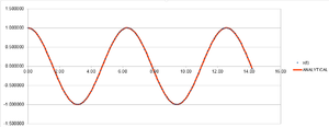


The Velocity-Verlet algorithm is a variant on the Verlet equation, in that it also takes the velocity of an atom into account.
NJ: They're actually completely equivalent formulations, its just that classic Verlet doesn't let you determine the atomic velocities. You don't need them for the simulation itself, but they're useful to have if you want to work our temperatures.
It can be used in this sense to work out the position of an atom in a classical harmonic oscillator scenario. Using the data provided in the HO.xls file, through the HPC facilities, it is possible to quantitatively analyse the equation.
The output graphs included cosine type curves for both the Analytical vs. T and the Energy vs. T as can be seen in figures 1 and 2. Figure 3 shows the Error vs. T graph, which can be seen to increase as time increase. The reasoning behind this is due to the fact that the Verlet-velocity involves a Taylor series, which often has an increase in error as the number of calculations made using it increase. The maximum error however is very low, at only 0.6% according to the calculated error. This helps suggest to us that the equation at the given timestep of 0.1 gives an acceptable idea of the physical behaviour of the physical system due to the low error. Of course, a lower error would be preferable, but given the inherent error of the Taylor series, the Velocity-Verlet equation can be considered to be relatively accurate.
Simply by using an iterative (trial and error) method, it is possible to see that at a lower timestep the error produced is smaller than it is at a higher timestep. This in itself makes sense as the time being analysed is smaller, and the distance in which a particle can move within the time given for the timestep is less. However, the timestep that is initially used, 0.1s, actually has an error of less than 1%, and so it is possible to increase the timestep in order to get reasonable results which have a longer time period of analysis. Analysing different values, you can see which timestep will give an error of 1%, and so is the maximum possible, which is 0.12 seconds. This process - the analysis of error - is vital during the running of such a simulation as you may appear to have results which deviate hugely from the theory with limited idea as to why if the error was not kept in check. If the error simulation is run at the same time we can see at which time we should disregard the results we receive - particularly important during long scale simulations.
NJ: Careful, these are reduced units - not seconds. People usually find 0.2 is the largest acceptable error, did you include the potential energy in your calculation?
Atomic Forces
The classical (or ideal) view of particles as small, hard points which feel no repulsion from one another before they have collided has to be completely disregarded when discussing the way in which real particles (atoms or molecules) act whilst in a system. The interactions that these particles actually experience is predominantly described by the Lennard-Jones potential. Using the equation for the potential with respect to r, it is possible to determine the separation of two atoms when they have a zero potential energy. This can also be determined graphically as the point at which the curve crosses zero. In general, this can be described algebraically to have a general answer of r = σ. When the particles are at this separation, the force between them is repulsive due to the fact that they are so close together. This makes sense, looking at the Lennard-Jones plot, as the point at which r = σ has a large negative potential next to it, which of course is a state in which the particles would prefer to be. This state can also be known as the equilibrium separation.
The equilibrium separation, req, is directly related to the well depth, Φ(req) or ε, as being the lowest possible potential energy of two particles interacting with one another. It is possible to use the idea that there is no force at req due to the fact that it is at equilibrium to give us an algebraic value for the separation as . We can input this into the Lennard-Jones equation to get a result for the well depth, .
If we take , we can integrate the Lennard-Jones potential with the limits of infinity to 2σ, 2.5σ and 3σ, then it is possible to determine definite integrals. The results of these integrations are -0.0248, -0.00818 and -0.00329 respectively. It perhaps isn't a huge stretch of imagination to consider the fact that at infinite separation the interaction between the two atoms would be zero, which is true, as the interaction between the two atoms appears to decrease as σ increases. NJ: The well depth is actually -epsilon. Everything else here is correct, although I would like to see working!
Periodic Boundary Conditions
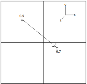
Almost all systems are imagined in the sense of lattices - certainly the starting point of the simulation previously run had all of the atoms in a regular lattice that then collapsed once the reaction had begun.
To visualise how many atoms there are in a system, it is useful to imagine 1ml (or 1g) of water (). By using the molecular mass of 18 we get in 1ml of water. By doing the reverse, and taking the number of particles analysed in the previous sections, 10000, then it is easy to see how small the system that is being analysed is at .
It is obviously very difficult to visualise a 3D system on a 2D surface, such as a screen, and difficult to imagine a 3D system in your head. One way around this is to apply periodic boundary conditions (PBCs) which massively simplify this visualisation. The whole idea of these PBCs is that if a particle moves through a lattice, to the edge of the box, it will move through to the other box. The different box is something formed during the "unfolding" of the 3D lattice. It can be visualised below in figure 5, in which an atom which had a position (0.5, 0.5, 0.5) in a box that runs from (0, 0, 0) to (1, 1, 1) moves along a vector of (0.7, 0.6, 0.2) in a single timestep then it will end up at the position of (0.2, 0.1, 0.7).
NJ: It's not to do with visualisation - the computer can handle 3 dimensions easily enough. We need PBCs to avoid having an interface at the edge of the box.
Reduced Units
One major issue with the Lennard-Jones potential is the magnitude of the answers which are obtained are often at tricky magnitudes, which can appear to be impenetrable, but can be made more accessible by using an idea known as reduced units. These are often denoted by an asterisks, and can be used to extract the "real" information from. Using argon which has parameters of it is possible for us to look at a number of examples using the reduced unit calculations:
- If r*=3.2, what is r in real units?
- What is the well depth?
- . These units are directly equal to or Joules, and so by applying unit conversions of you get the well depth in . This is .
- What is the reduced temperature, T*=1.5, at an actual temperature?
As can be seen, the reduced units are easy to convert into the real units, and can prove to be exceptionally helpful at presenting clear and easy to vary data.
Equilibration
Running a LAMMPS simulation
When it is required to run a simulation of how particles move in a system it is required to use LAMMPS on the HPC. This is a code that is used for uses classical molecular dynamics to model the systems being run. The output for these can be either .log, which provide a lot of useful information on the energy, error, timestep etc. (it depends on what is analysed and printed), or .lammpstrj, which can be used in VMD to provide a visual outlook at the way the system runs.
When the simulation is run it is imagined to be in a regular lattice in order to simplify the generation of a box. The reason that the particles aren't generated in random places is due to the fact that there are a lot of particles in a finite space. The fact that the particles are in a finite space, and then randomly generated, would mean that with the number of particles, there is a high probability that two particles would be generated on top of, or very, very close, to one another. This is obviously not representative of a real system, especially if they are on top of one another as that is a physical impossibility. This would lead to inconsistent and odd results, as many particles would repel eachother strongly from the start, pushing them further away from one another as the simulation runs. This is particularly true if they are generated at a distance of less than .
Creating the simulation box
In the LAMMPS code that is provided, there is the line lattice sc 0.8. This corresponds to the density of the system, saying that there are 0.8 lattice points per unit cell. The side of the simple cubic lattice has a size (r*) of 1.07722, and so we can work out the density of the cell directly by using the equation:
It is also useful to consider different systems, as not every liquid will start with a simple cubic lattice at a density of 0.8! One possible starting point for the LAMMPS script is a face-centered cubic lattice at density 1.2. In a face centered lattice there are 4 atoms per unit cell, not just the 1 seen for a simple cubic lattice. The sides of the unit cell can be determined using these parameters, as well as the rearrangement of the previously used equation.
We can now consider that the total number of unit cells used in the simulation is the same as before. From this we can determine - due to the fact that the previous, simple cubic lattice, has 10 unit cells in all directions - how many atoms will be found in this simulation.
As the simple cubic lattice has 1000 atoms, with one atom per unit cell, this means there are 1000 unit cells in the simulation. As the face centered cubic lattice has 4 atoms per unit cell, and the simulation, this means that there are 4000 atoms in this face-centred cubic lattice simulation.
Setting Atomic Properties
In the input script for the LAMMPS simulation there are a number of key lines. Using the LAMMPS manual, it is possible to decipher what these actually mean:
mass 1 1.0- The
masscommand provides the mass for one, or all, of the atoms. The1 1.0corresponds to the allocation of a mass of 1.0 to just one atom.
- The
pair_style lj/cut 3.0- The
pair_style lj/cutis the cutoff for the Lennard-Jones potential with no Coulomb interaction.3.0refers to the the distance in r* at which the aforementioned cutoff will occur.
- The
pair_coeff * * 1.0 1.0- The
pair_coeffrelates to the pairwise forcefield coefficients. The* *set the commands for the I and J functions - the two types of atoms - and are known as wildcard asterisk's and so can be given any value.1.0 1.0define the pairwise forcefield coefficients for the I and J atom types.
- The
NJ: What do you mean by forcefield coefficients?
Throughout this simulation we are using and . This suggests that for the LAMMPS input code we are not using the Verlet algorithm, rather the velocity-Verlet algorithm.
Running the Simulation
When we go to run the simulation, we do not just want to specify the timestep and the number of runs, but rather, we want to keep the time the simulation runs for constant. This can be achieved by using an equal floor input, which will allow for the actual amount of time for which the simulation is run to be kept constant. This means that when it is imperative to compare the difference that timesteps can have on the output of data, it is possible to have a consistent scale, rather than a constantly changing scale.
Output
Following the running of the simulation on the HPC facilities, at a number of different timesteps (0.001, 0.0025, 0.0075 0.01 and 0.015) we receive the useful data. From this it is possible to determine if the simulation reaches equilibrium, and by comparing the different results given by the timesteps, we can see which timestep is appropriate to run the other simulations at in order to provide good results using the least possible time and computer power.
 |
 |
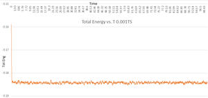 |
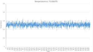
As you can see from the Energy vs. T, Pressure vs. T and Temperature vs. T graphs for the 0.001 timestep simulation, the system very quickly reaches equilibrium - in 0.41 "time units", and whilst there are fluctuations about the equilibrium, this is to be expected in any sort of equilibria. It is also important to note that the energy of the 0.001TS system has dropped into a negative energy which is very important due to the fact that according to the Lennard-Jones potential, the energy should collapse into a negative value when the particles are at .
NJ: The potential energy will. Remember that you have kinetic energy too!

Looking at the graph which displays all of the different Total Energy vs. T outputs for the different timesteps, you can see which reach equilibria. Four of the run timesteps do, with 0.001 and 0.0025 being the most accurate (as they are at the lowest energy). Taking into account what was said earlier about time taken and computer power, this suggests that the best timestep to run the simulation at isn't the smallest - 0.001 - but is instead 0.0025 due to the lack of change in Energy, and the larger timestep. This should decrease the amount of time and computer power used (or certainly the number of data points to analyse!!) by two and a half times. Therefore 0.0025 is the largest acceptable timestep.
There is however, a particularly unacceptable timestep visible on the graph, that of 0.015. This is so far off the energy that it doesn't actually appear to reach equilibrium. The black line on the graph which represents it goes in a completely different direction to the rest of the lines on the graph, increasing after it is reduced, suggesting that the results being given are incorrect. Therefore, despite the small simulation time, it is not at all advisable to use 0.015 as your timestep when running this simulation.
Running simulations under specific conditions
By analysing the pressure vs. Time graph from the previous section we can create a number of differing input files for npt.in. The average pressure can be seen to be about 2.6, so two values of 2.55 and 2.65 should be satisfactory to provide differing, but accurate results for use in the input files. The five temperatures chosen are 1.6, 1.7, 1.8, 2.0 and 3.0. This is to provide a small series, as well as one temperature that has wildly varied from the others, all about 1.5, to be able to extract the maximum amount of information from the small number of data points being investigated.
In the input file, there is a set of code under the name ### MEASURE SYSTEM STATE ###. The final line of this part of the code has a section as such:
fix aves all ave/time 100 1000 100000
These three numbers have three different key functions:
100- Every 100 timesteps use the input values.
1000- The total number of times this should be done is 1000.
100000- Every 100000 timesteps, calculate the average values.
This means that using the timestep of 0.0025 determined in the previous section, the simulation will run for 250 time units.
Thermostats
When we run a simulation, the temperature is constantly changing. This can be seen in the Temperature vs. Time graph from the previous section, with there being fluctuations about the equilibrium temperature. This temperature is defined as the desired temperature, , whilst the temperature at any given any given moment is the instantaneous temperature, .
It is possible to rectify this by using the correcting variable which corrects the velocity in the simple kinetic energy equation. This value has to be able to vary as it has to be able to correct the temperature more if it is further from the target temperature than it does if it is at .
Simple rearrangement of two equations - one including and , and the other and . By cancelling out the equal terms of these two equations we get:

Output
The output of this code gives us the values and error of pressure, p, temperature, T, and density, or .
As you can see from the graph, the simulations that ran at the pressures of 2.55 and 2.65 are both very similar in density as temperature varies. However, the 2.65 curve is higher than the 2.55 curve, which is in line with what is expected for this graph. The error is quite large, but this is to be expected with such a calculation of many thousands of particles.
NJ: Actually, the more particles you have, the more accurate the results will be. You have more contributions to the calculation of temperature and pressure.
The ideal gas calculations show this discrepancy to a much larger extent. They are calculated using the equation:
However, throughout this experiment we are using number values and so can be disregarded, as can be put in reduced values, so equals one to give:
The simulated density is lower than the ideal gas law calculations for a relatively simple reason. The ideal gas law imagines particles are small points which do not interact with eachother in any sense other than when they hit eachother. This means that the particles in the ideal gas law can get closer together than the real particles, which experience potential energy too, in the sense of repulsion. This is described by the Lennard-Jones potential in the way that the potential, repulsive energy goes to infinity as r tends to 0. This means that the particles in the actual simulation cannot touch and instead repel eachother well before this point. Assuming the particles for the ideal and real systems are the same size, and there are the same number of particles in both systems, the ideal particles can occupy a smaller volume than the real particles, making the ideal system denser.
The higher pressure system shows this in a more pronounced fashion, with there being a larger discrepancy between the real 2.65 and ideal 2.65, than there is between the real and ideal 2.55 pressure system. This is because not only are the ideal particles forced closer together, but the real particles are as well and so they experience a greater repulsion, pushing them apart from one another.
As the temperature of the system increases then the density decreases. This is due to the fact that the particles have more energy and so are pushed further apart from one another as they have more energy. This increase in kinetic energy means that the particles are more likely to collide and fly away from one another, which once again decreases the density.
Calculating heat capacities using statistical physics
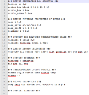
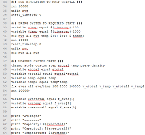
It is possible to alter the input script from the previous section to calculate the heat capacity. An example of such an input script is shown in two parts.
This provides three key outputs; average temperature; average energy; and average energy squared. These can all be used in the equation for heat capacity, where is the number of particles in the system:
It is then vital to determine the volume of the simulation box. As the lattice sides are 15 in a simple cubic lattice:
There is only one value left to find, which is that of the number of particles in the simulation. This is a case of finding the product of the density and the volume, to give two values:
- For =0.2:
- atoms
- For =0.8
- atoms
NJ: I'm afraid not - you should divide by the volume. At the moment, your higher density system has a larger volume for the same number of atoms. You can also get this directly from the simulation log file.
These two values can then be inputted into their respective equations in order to find appropriate values for .
Analysis through excel produces the following graph:
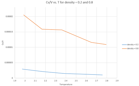
The general definition of heat capacity is the amount of energy required to heat 1 mole of a substance by 1 degree Celsius. If there is an increase in temperature, and density and volume are held constant, then the particles are more excited and so the capacity should increase. However, this is not what is observed. Instead, it is observed that the value decreases. This suggests that the input code may not be perfect.
This discrepancy is far more prevalent in the more dense system, which is logical as the particles are closer together (and more abundant) in this dense system, meaning that energy is transferred to them with greater ease. This results in greater values for the capacity being used and so a greater error being observed.
Structural properties and the radial distribution function
The radial distribution function for a solid, liquid and vapour system were determined using a Lennard-Jones phase diagram. This gave:
- Gas
- =0.01, T=1
- Liquid
- =0.8, T=1
- Solid
- =1.2, T=1
Using VMD we were able to calculate the RDF (g(r)) and its integral (int(g(r))) and plot them in excel.
 |
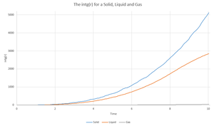 |

In the Radial distribution function, the more peaks there are visible on the plot, the more long range ordering you have. This can be seen on the plot for the solid, liquid and gas simulations. It makes sense that the solid has more ordering than the liquid, and the liquid has more ordering than the gas due to the very nature of the systems. It can be noted that the solid RDF has more peaks that the liquid RDF etc. which suggests that the more peaks there are in a RDF plot, the higher the long range ordering.
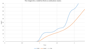
As the solid has a face-centered cubic lattice structure, unlike the liquid and gas which are simple cubic lattices (denoted in the input script by fcc rather than sc) then the first three solid peaks on the RDF graph denote the following lattice sites:
The dark blue atom corresponds to the reference atom and so has no peak. The yellow atoms are the atoms which correspond to the first peak and are at a distance of where is the length of a unit cell side. The green atoms correspond to the second, small peak, and are at a distance of from the reference atom. The third peak is produced upon interaction of the reference atom with the red lattice sites. These are at a distance of from the dark blue lattice site.
It is possible to determine in terms of reduced units, which gives us the lattice spacing. As this is a face-centered cubic lattice, and the input file had density, , set to be 1.2, then it can be determined that is equal to:
Using a zoomed in version of the int(g(r)) graph it is possible to determine the coordination states about the lattice sites discussed previously. The point at which the curve plateaus is the point at which the coordination number can be determined. By looking at the y-value you have the total number of co-ordination points from the reference lattice space, so you can take the previous plateau's y-value from that determined to find the co-ordination number for the first 3 peaks. These are, in order 12 for the yellow lattice sites, 6 for the green lattice sites and 24 for the red lattice sites.
NJ: Nice analysis. You could also have read the lattice spacing from the log file - unfortunately, I wanted you to work it our by looking at the positions of the peaks in the RDF.
Dynamical properties and the diffusion coefficient
Running a simulation in order to find the mean squared displacement and velocity autocorrelation function of a solid, liquid and gas system, has a timestep of 0.002 and the following input densities and temperatures:
- Gas
- =0.4 T=1.3
- Liquid
- =0.9 T=1
- Solid
- =1.2 T=1.2
NJ: The temperature and density are possibly a bit high for the gas. You might be in the fluid region. I appreciate that it's very hard to pick a gas state point from that old phase diagram.
Mean Squared Displacement
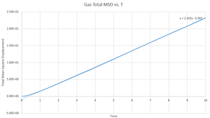
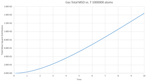
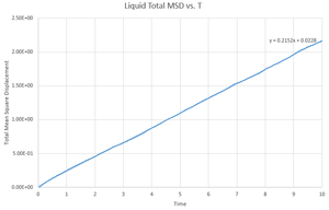
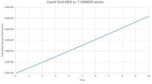
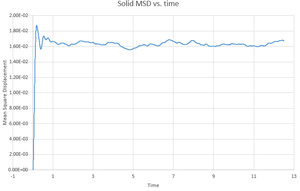
This gives the output files which can be seen below, along with a simulation of the mean square displacement with 1,000,000 atoms. The gradient of these curves can be used to find the Diffusion coefficient, :
The values for are determined using the trendline function on Excel and analysing its gradient.
 |
 |
 |
 |
 |
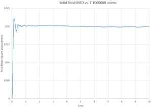 |
The deviation between the 1,000,000 atom systems and the lower atom systems is obvious - each of the 1,000,000 D values are higher than the lower atom D values. This makes sense as there are more chances for a collision in the 1,000,000 atoms system and so the chance for random motion is much higher.
NJ: That's not it. If the two simulations are under the same conditions, then the 10^6 atom simulation will give you much more accurate results. However, do you know what conditions I chose for the 10^6 atom simulation...?
Velocity Autocorrelation Function
Integration of VACF for 1D harmonic oscillator
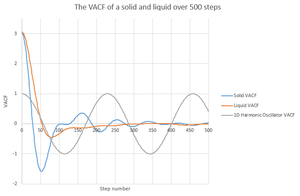
VACF plot
Using and the VACF outputs from the simulations that were previously run, it is possible to plot graphs for .
The minima on this plot represent the change in direction of the velocity to one that is negative. The predominate reason for the differences between the solid and liquid VACF plots is that the solid particles cannot move with the same ease of the liquid particles and so it is far more correlated to the particle it hit amount of time ago than the liquids, which very quickly lose such correlation.
NJ: The first minimum for the liquid is often attributed to the collision with the solvent cage.
The harmonic oscillator VACF is in just one dimension, whilst all of the other simulations consider the three dimensions. The particle that can only move in one direction which means that it cannot move, and so it doesn't lose its correlation coefficient.
NJ: That's not the reason - your answer doesn't really make sense. The key is that the harmonic oscillator doesn't have anything to "collide" with to decorrelate its velocity.
Estimates of D
- Solid
- Using the trapezium rule it is possible to get an estimate as to the area under the VACS curve, and then, multiplying by an estimate can be made for the value of .
- Liquid
- The trapezium rule gives a value of 50.27846.
- Gas
- The trapezium rule gives a value of 534.2267.
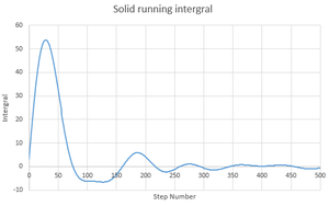
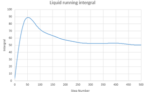
By plotting the running integrals for the solid, liquid and gas states of the system, it is possible to see if they act in the way that is expected:
 |
 |
 |
The solid and liquid not act in a way that is expected. If they did then we would see a constant increase as is seen in the gas running integral. Instead there is a fluctuation as the number of steps increases as there are negative values. They do however, give the same final value.
Estimates for D for 1,000,000 atom systems
- Solid
- The trapezium rule gives a value of -0.41627
- Liquid
- The trapezium rule gives a value of 123.7271
- Gas
- The trapezium rule gives a value of 1466.443
 |
 |
 |
There are large discrepancies between the values for for both the 1,000,000 and lower atom systems. This is most likely due to the large inherent error of the trapezium rule in comparison to the high accuracy of the differential. There is however the same general trend of the solid having the smallest diffusion coefficient and the gas having the largest. Whilst the values for are many orders of magnitudes off one another, they can be both considered, in their own respect, to be accurate.
NJ: The trapezium rule wouldn't give you an error or orders of magnitude. However, you've worked out D in terms of distance^2 per timestep for the VACF. For the MSD you worked out distance^2 per time. The two sets of values therefore differ by approximately
