Simulation of a Simple Liquid

Introduction to Molecular Dynamic Simulation

TASK: Open the file HO.xls. In it, the velocity-Verlet algorithm is used to model the behaviour of a classical harmonic oscillator. Complete the three columns "ANALYTICAL", "ERROR", and "ENERGY": "ANALYTICAL" should contain the value of the classical solution for the position at time $t$ , "ERROR" should contain the absolute difference between "ANALYTICAL" and the velocity-Verlet solution (i.e. ERROR should always be positive -- make sure you leave the half step rows blank!), and "ENERGY" should contain the total energy of the oscillator for the velocity-Verlet solution. Remember that the position of a classical harmonic oscillator is given by $x (t) = A \cos (ω t + ϕ)$ (the values of $A$ , $ω$ , and $ϕ$ are worked out for you in the sheet).

The graphs on the side compare the difference in results between the simulated oscillator from the velocity-Verlet solution and the calculated data on a classical harmonic oscillator. They also formulate the difference generated between the two oscillating systems as error.

The graph, fig.3, shows the absolute error of the difference between the calculated values of the position of the atom in the harmonic oscillator compared to the simulated values of the position as a function of time. Here, the trend line keeps reverting back to zero, this is due to the intrinsic property of the oscillator. When the simulated and the analytical oscillator are oscillating at the same time, their difference will become larger as the analytical oscillator is faster and will increase the error in displacement. However as time moves on the faster oscillator will lap the slower one and close in on the difference in displacement. This is why the graph reverts back to the value zero periodically. It is not because there is no error between the two oscillators. The overall trend in the graph shows that the error is accumulative overtime and this is why the maxima in each period increases.

TASK: For the default timestep value, 0.1, estimate the positions of the maxima in the ERROR column as a function of time. Make a plot showing these values as a function of time, and fit an appropriate function to the data.

Fig.4 has plotted the maxima in fig.3 as a function of time. It shows how the overall absolute error generated between the two oscillating systems is increasing. This trend means that error in this system is accumulative over time and how the simulated values deviated further and further from the calculated analytical values.

TASK: Experiment with different values of the timestep. What sort of a timestep do you need to use to ensure that the total energy does not change by more than 1% over the course of your "simulation"? Why do you think it is important to monitor the total energy of a physical system when modelling its behaviour numerically?

The largest timestep that ensures the total energy does not change by more than 1% is 0.20. Through excel calculations, the change in total energy is easily monitored when the timestep is changed. At a timestep of 0.20, the energy changed from 0.500 to 0.495. The change in timestep usually introduces error into the detection of total energy in the system. For instance a larger timestep increases the time intervals between detection and this will monitor a larger difference in the change in energy compared to a smaller timestep. When the total energy of a physical system can be monitored then the outcomes of the simulation can be checked upon. If there was a sudden or irregular change in the total energy then the problem can be immediately identified. NJ: Because we know that the law of conservation of energy has to be satisfied.

TASK: For a single Lennard-Jones interaction, $ϕ (r) = 4 ϵ (\frac{σ^{12}}{r^{12}} - \frac{σ^{6}}{r^{6}})$ , find the separation, $r_{0}$ , at which the potential energy is zero. What is the force at this separation? Find the equilibrium separation, $r_{e q}$ , and work out the well depth ( $ϕ (r_{e q})$ ). Evaluate the integrals $\int_{2 σ}^{\infty} ϕ (r) d r$ , $\int_{2.5 σ}^{\infty} ϕ (r) d r$ , and $\int_{3 σ}^{\infty} ϕ (r) d r$ when $σ = ϵ = 1.0$ .

TASK: Estimate the number of water molecules in 1ml of water under standard conditions. Estimate the volume of $10000$ water molecules under standard conditions.

TASK: Consider an atom at position $(0.5, 0.5, 0.5)$ in a cubic simulation box which runs from $(0, 0, 0)$ to $(1, 1, 1)$ . In a single timestep, it moves along the vector $(0.7, 0.6, 0.2)$ . At what point does it end up, after the periodic boundary conditions have been applied?.

By moving the atom along the vector $(0.7, 0.6, 0.2)$ , the atom will end up at $(1.2, 1.1, 0.7)$ . However since the since one unit cell is 1 unit in all three dimensions, this is not possible. Due to periodic boundary conditions, the atom that exists the box will be replicated at the other end of the box, hence the final position of the atom should be at $(0.2, 0.1, 0.7)$ .

TASK: The Lennard-Jones parameters for argon are $σ = 0.34 n m, ϵ / k_{B} = 120 K$ . If the LJ cutoff is $r^{*} = 3.2$ , what is it in real units? What is the well depth in ${k J m o l}^{- 1}$ ? What is the reduced temperature $T^{*} = 1.5$ in real units?

Equilibration

TASK: Why do you think giving atoms random starting coordinates causes problems in simulations? Hint: what happens if two atoms happen to be generated close together?

When two atoms are generated close together the potential energy generated with the atoms’ placement will be very large and the atoms will be pushed apart with a large velocity and potentially colliding with other atoms. This will create simulation system with a larger disorder with a very large initial energy. The problem is worsened due to periodic boundary conditions. In the system, the atoms are all enclosed inside a cubic box which is repeated infinitely in 3 dimensions. However when an atom reaches the boundary of the simulation box, a replica of it is produced at the other side of the simulation box so that the total number of atoms inside the box will remain constant. This condition is called periodic boundary conditions. When this constantly happens due to many atoms traveling at a high velocity caused by close placement when generated, it will interfere with the conditions and dynamics set for the simulation, meaning that the data in the output files are not reporting on accurate data.

TASK: Satisfy yourself that this lattice spacing corresponds to a number density of lattice points of $0.8$ . Consider instead a face-centred cubic lattice with a lattice point number density of 1.2. What is the side length of the cubic unit cell?

TASK: Consider again the face-centred cubic lattice from the previous task. How many atoms would be created by the create_atoms command if you had defined that lattice instead?

In a face-centred cubic lattice, there would be 4,000 atoms. There are 4 atoms per unit cell and the initial conditions have set for a simulation box with 1000 lattice unit cells. (10 x 10 x 10 as shown below.)

region box block 0 10 0 10 0 10
create_box 1 box

TASK: Using the LAMMPS manual, find the purpose of the following commands in the input script:

mass 1 1.0
pair_style lj/cut 3.0
pair_coeff * * 1.0 1.0

Mass 1 1.0 defines the mass for all the atoms, and in this case there is only one type of atom in the system, hence all the atoms will have the same mass, which is 1.0 in reduced units.

pair_style lj determines the potential between the particles, in this case it is the Lennard Jones Potential. cut 3.0 means that any two particles 3 $σ$ or more apart will have negligible interaction, and will be set to zero.

pair_coeff * * 1.0 1.0 determines the well depth $ϵ$ and the distance at which the inter-particle potential is zero $σ$ , the two parameters in the Lennard Jones potential. NJ: Good

TASK: Given that we are specifying $x_{i} (0)$ and $v_{i} (0)$ , which integration algorithm are we going to use?

The Velocity Verlet Algorithm is an improvement on the Verlet Algorithm. It integrates Newton's equations and takes the velocity into account, which can be then be used to calculate the kinetic energy.

TASK: Look at the lines below.

### SPECIFY TIMESTEP ###
variable timestep equal 0.001
variable n_steps equal floor(100/${timestep})
variable n_steps equal floor(100/0.001)
timestep ${timestep}
timestep 0.001

### RUN SIMULATION ###
run ${n_steps}
run 100000

The second line (starting "variable timestep...") tells LAMMPS that if it encounters the text ${timestep} on a subsequent line, it should replace it by the value given. In this case, the value ${timestep} is always replaced by 0.001. In light of this, what do you think the purpose of these lines is? Why not just write:

timestep 0.001
run 100000

The purposes of the lines is that the total amount of simulated time in reduced units remain constant despite changing the timestep. Therefore, the number of timesteps simulated in the above diagram is 100,000. However the total number of simulated time is 100 reduced units. On the other hand if the timestep is changed, the number of timesteps simulated will change accordingly so that the total simulated time will always remain 100 reduced units.

NJ: Excellent

TASK: make plots of the energy, temperature, and pressure, against time for the 0.001 timestep experiment (attach a picture to your report). Does the simulation reach equilibrium? How long does this take? When you have done this, make a single plot which shows the energy versus time for all of the timesteps (again, attach a picture to your report). Choosing a timestep is a balancing act: the shorter the timestep, the more accurately the results of your simulation will reflect the physical reality; short timesteps, however, mean that the same number of simulation steps cover a shorter amount of actual time, and this is very unhelpful if the process you want to study requires observation over a long time. Of the five timesteps that you used, which is the largest to give acceptable results? Which one of the five is a particularly bad choice? Why?

Yes the simulation reaches equilibration. The max point and the min point in the first period of the Energy graph was found through the simulated outcomes, an average of the Energy was taken using the two (-3.1843963, and -3.1835095) to give a value of -3.183953 and the time it took to reach equilibration was 0.36 seconds.

NJ: Be careful with units, these should be reduced.

The 0.0025 would be a good compromise between not taking too many time steps but still giving an accurate enough set of data since the data it shows is almost overlapping with 0.001 (the most accurate results), but takes less processing power compared to 0.001. As the graph below shows, the smaller the timestep the lower the total energy was over time. The smallest timestep 0.001 takes the most number of timesteps and represents the most accurate set of results, however it will also take the longest processing time to simulate the same amount of real time.

On the other hand it seems that the frequency of the timestep affects the total energy observed. The larger the timestep (the less frequent detection happens during the simulation) the less accurate the recorded total energy becomes. The worst choice of the five is the 0.015 timestep, which is the largest timestep. It deviates from the data shown by the other four sets of data by increasing in an almost linear manner while fluctuating. The data shown by 0.015 seems that at such a low frequency of measurement of the total energy, that the total energy would increase overtime. Apparently a large timestep would cause a molecular simulation to become unstable because it would sometimes measure the position of two atoms to be overlapping and assume that devastating atomic collisions were occurring. Hence the total energy would increase by large amounts over time. The 0.015 graph also shows that error is accumulative over the time of the simulation. This is why the value of the total energy deviates more and more from the values generated from smaller values of timestep.

Running Simulations Under Specific Conditions

TASK: Choose 5 temperatures (above the critical temperature $T^{*} = 1.5$ ), and two pressures (you can get a good idea of what a reasonable pressure is in Lennard-Jones units by looking at the average pressure of your simulations from the last section). This gives ten phase points — five temperatures at each pressure. Create 10 copies of npt.in, and modify each to run a simulation at one of your chosen $(p, T)$ points. You should be able to use the results of the previous section to choose a timestep. Submit these ten jobs to the HPC portal. While you wait for them to finish, you should read the next section.

Pressure	Temperature
2.75	1.6	1.8	2.0	2.5	3.5
2.6	1.6	1.8	2.0	2.5	3.5

TASK: We need to choose $γ$ so that the temperature is correct $T = 𝔗$ if we multiply every velocity $γ$ . We can write two equations:

$\frac{1}{2} \sum_{i} m_{i} v_{i}^{2} = \frac{3}{2} N k_{B} T$

$\frac{1}{2} \sum_{i} m_{i} {(γ v_{i})}^{2} = \frac{3}{2} N k_{B} 𝔗$

Solve these to determine $γ$ .

TASK: Use the manual page to find out the importance of the three numbers 100 1000 100000. How often will values of the temperature, etc., be sampled for the average? How many measurements contribute to the average? Looking to the following line, how much time will you simulate?

Nevery takes the input value every 100 timesteps. The number of measurements that contribute to the average is calculated over Nrepeat number of values, which is 1000 values. The values of temperature will be sampled every Nfrequency, which is 100,000 number of steps. This means that at 100,000 time step, an average is taken across 1000 values at 99,900, 99,800, 99,700...etc.

The importance of these three numbers shows how the average values are calculated for a simulated box by selecting data from the total values evaluated in all the timesteps.

The total time simulated depends on the timestep chosen. In this case it is 0.0025. $0.0025 * 100, 000 = 250$ time in reduced units

TASK: When your simulations have finished, download the log files as before. At the end of the log file, LAMMPS will output the values and errors for the pressure, temperature, and density $(\frac{N}{V})$ . Use software of your choice to plot the density as a function of temperature for both of the pressures that you simulated. Your graph(s) should include error bars in both the x and y directions. You should also include a line corresponding to the density predicted by the ideal gas law at that pressure. Is your simulated density lower or higher? Justify this. Does the discrepancy increase or decrease with pressure?

The graphs on the right have been created by plotting density as a function of temperature at constant pressure. The values of density are measured by simulation and by calculation using the Ideal Gas Law.

Both the simulated density and the ideal gas law density decrease as temperature increases because as there is more energy in the system the atoms will gain more vibrational energy and move from their equilibrium position. Both densities also increase with increasing pressure. The ideal gas law densities are higher because the kinetic theory assumes that any interaction between particles is zero, hence particles can be packed tighter together. At the same when the Lennard Jones particles are packed together, they will experience high potential energy which creates repulsion, hence the density is lower.

Pressure	Input Temperature	Density	Pressure	Input Temperature	Density
2.60	1.6	1.63	2.75	1.6	1.72
	1.8	1.44		1.8	1.53
	2.0	1.30		2.0	1.38
	2.5	1.04		2.5	1.10
	3.5	0.742		3.5	0.786

The error bars are calculated from simulations and plotted into the graphs. Only the ones for temperature show up as the ones for density are too small to be noticed. It is worth mentioning that the error bars increase as temperature increase. This is because at a higher temperature the temperature will fluctuate more and hence introduce a larger error for measurement.

Lastly the difference between simulated values and ideal gas law values decreases as temperature increases because higher temperature creates a lot of kinetic energy, which overcomes the potential energy creating repulsive forces. By removing the potential energy barrier(repulsive forces), the Lennard Jones particles have a higher density at a higher temperature. This is why the discrepancies between the two sets of data decrease over higher temperature.

NJ: Good. How does the agreement change with pressure?

Calculating Heat Capacities using Statistical Physics

TASK: As in the last section, you need to run simulations at ten phase points. In this section, we will be in density-temperature

$(ρ^{*}, T^{*})$

phase space, rather than pressure-temperature phase space. The two densities required at

$0.2$

and

$0.8$

, and the temperature range is

$2.0, 2.2, 2.4, 2.6, 2.8$

. Plot

$C_{V} / V$

as a function of temperature, where

$V$

is the volume of the simulation cell, for both of your densities (on the same graph). Is the trend the one you would expect? Attach an example of one of your input scripts to your report.

The graph on the right, fig.11, shows how as density increases the heat capacity increases. Under a NVT system, this would be because a higher density means there are more molecules in the same volume and hence there are more degrees of freedom. Therefore more energy would be required to increase the temperature by one unit. NJ: Heat capacity is extensive

Both the trends show how the heat capacity decreases as the temperature increases. In quantum mechanics the excited energy levels converge from the ground state, so less energy input is required as the liquid is simulated from a more excited energy level each time. Therefore the heat capacity to increase the energy level of the liquid will decrease every time.

NJ:Careful, this system is classical. You can extend the ideas about "modes" to this system though.

The point at temperature 2.4 is an anomalous data.

This is because the “12345” script input from:

velocity all create ${T} 12345 dist gaussian rot yes mom yes

This means that the velocity in the system is randomly generated, which means it is possible to generate errors, but the size of the errors are unknown.

Example Script for calculating the heat capacity and heat capacity/volume:

### DEFINE SIMULATION BOX GEOMETRY ###
lattice sc 0.2
region box block 0 15 0 15 0 15
create_box 1 box
create_atoms 1 box

### DEFINE PHYSICAL PROPERTIES OF ATOMS ###
mass 1 1.0
pair_style lj/cut/opt 3.0
pair_coeff 1 1 1.0 1.0
neighbor 2.0 bin

### SPECIFY THE REQUIRED THERMODYNAMIC STATE ###
variable T equal 2.2
variable timestep equal 0.0025 

### ASSIGN ATOMIC VELOCITIES ###
velocity all create ${T} 12345 dist gaussian rot yes mom yes

### SPECIFY ENSEMBLE ###
timestep ${timestep}
fix nve all nve

### THERMODYNAMIC OUTPUT CONTROL ###
thermo_style custom time etotal temp press
thermo 10

### RECORD TRAJECTORY ###
dump traj all custom 1000 output-1 id x y z

### SPECIFY TIMESTEP ###

### RUN SIMULATION TO MELT CRYSTAL ###
run 10000
unfix nve
reset_timestep 0

### BRING SYSTEM TO REQUIRED STATE ###
variable tdamp equal ${timestep}*100
variable pdamp equal ${timestep}*1000
fix nvt all nvt temp ${T} ${T} ${tdamp}
run 10000
reset_timestep 0

###Switch off the thermostat with the commands###
unfix nvt
fix nve all nve

### MEASURE SYSTEM STATE ###
thermo_style custom step etotal temp press density
variable temp equal temp
variable temp2 equal temp*temp
variable etotal equal etotal
variable etotal2 equal etotal*etotal
variable atoms equal atoms
variable N2 equal atoms*atoms
variable vol equal vol
variable dens equal atoms/vol
fix aves all ave/time 100 1000 100000 v_temp v_etotal v_etotal2 v_atoms v_vol v_dens
run 100000

variable avetemp equal f_aves[1]
variable aveetotal equal f_aves[2]
variable aveetotal2 equal f_aves[3] 
variable aveatoms equal f_aves[4]
variable avevol equal f_aves[5] 

variable aveCv_V equal ${N2}*(f_aves[3]-f_aves[2]^2)/${temp2}/f_aves[5] 

print "Averages"
print "--------"
print "Cv/V: ${aveCv_V}"
print "Temperature: ${avetemp}"
print "etotal: ${aveetotal}"
print "etotal2: ${aveetotal2}"
print "atoms: ${aveatoms}"
print "vol: ${avevol}"

Structural Properties and the Radial Distribution Function

TASK: perform simulations of the Lennard-Jones system in the three phases. When each is complete, download the trajectory and calculate $g (r)$ and $\int g (r) d r$ . Plot the RDFs for the three systems on the same axes, and attach a copy to your report. Discuss qualitatively the differences between the three RDFs, and what this tells you about the structure of the system in each phase. In the solid case, illustrate which lattice sites the first three peaks correspond to. What is the lattice spacing? What is the coordination number for each of the first three peaks?

The following table shows the conditions under which the simulations of the Lennard-Jones system were performed.

	Temperature	Density
Solid	1.2	1.3
Liquid	1.3	0.82
Gas	1.2	0.05

The radial distribution function for Ar in gas, liquid and solid graph shows many peaks for solid state and few for liquid and only one for gas. Each peak shows the correlation of the density (to find a pair of atoms) around an atom with the distance in its radial space. The difference in the number of peaks show how in the solid there is long range order in the lattice structure of the solid however in the liquid there is only local structure and anywhere further becomes difficult to discern the density/structure. For gas there is only immediate surrounding order that can be accounted for and then it decays to a constant value at a distance. The peaks in the graph shows that the gas simulation plotted the broadest peak, this is expected since a broader peak indicates thermal motion, while the solid displayed the sharpest peak, indicating a strongly ordered structure where atoms are confined in their positions.

The radial distribution function has removed the $4 π r^{2}$ and divided by the bulk number density, thus calculating the probability of finding a pair of atoms at a distance. This function will tend to unity at large r.

The face centred cubic structure has 4 lattice points and all the atoms are in the same environment. The first peak shows the closest 12 atoms in the FCC structure. These 12 atoms are closest to the reference atom, at a distance of 1.025 reduced units, and because they are the closest, they also have the highest probability of being found. This number corresponds to the integral graph which shows 12 atoms at the plateau at a distance of 1.175 reduced units.

Image.2 shoes the 6 second closest atoms Ref. 2

When the lattice spacing is worked from the distance of the first peak using the Pythagorean Theorem, it is 1.414 in reduced units, this corresponds to the second peak at 1.475 in reduced units. This means that the group of second closest atoms are the 6 atoms that are one lattice spacing away from the reference atom. The integral of the graph shows a value of 18 for the second peak. This is because the number of atoms in the integral are cumulative, and hence confirms that the second closest atoms are 1.475 reduced units away. NJ: You could average the values of a from the three different peaks to get a more accurate result.

Using the distance to the first closest atoms and the lattice spacing(second closest atoms) in Pythagorean Theorem, the distance for the third closest group of atoms is at 1.796 in reduced units. This matches with the data from the g(r) graph: the third peak is at 1.775 in reduced units. The integral graph shows a value of 42.24, and this means that there are 42-12-6= 24 atoms that are third closest to the reference atom.

Image.3 shows the 24 third closest atoms Ref. 2

Distance	Distance (reduced units)	Coordination Number
First Closest	1.025	12
Second Closest	1.475	6
Third Closest	1.775	24

Dynamical Properties and the Diffusion Coefficient

TASK: make a plot for each of your simulations (solid, liquid, and gas), showing the mean squared displacement (the "total" MSD) as a function of timestep. Are these as you would expect? Estimate $D$ in each case. Be careful with the units! Repeat this procedure for the MSD data that you were given from the one million atom simulations.

D from MSD	Solid	Liquid	Gas
Simulated Data	$3.33 * 1 0^{- 6}$	$0.0845$	$2.54$
1 Million Atom Data	$5 * 1 0^{- 6}$	$0.0872$	$2.54$

The units of the diffusion coefficient, D, is in distance squared/ time in reduced units. The table above shows that the diffusion coefficient matches up well for the simulated data compared to the data simulated from 1 million atoms.

The mean squared displacement graphs show how much a reference particle has traveled in a certain time frame through Brownian motion. The diffusion constant for gas is very large, this shows how much a reference particle has travelled throughout the timeframe. This is expected since the gas state does not have much intermolecular interactions and hence particles are free to travel in the simulation box. In addition the gas graph shows a linear function, which indicates that not many molecular collisions have occurred such that it doesn't deviate from the path on a straight line.

NJ: The vapour results are noticeably curved.

The diffusion constant for the liquid is smaller, this shows how a liquid particle can travel but its movement is still restricted due to a somewhat ordered structure in its immediate environment. The graph is not a straight line and is typical of liquid MSD graphs as it shows particle collision occurring to deviate the traveled distance from a straight line plot. The diffusion constant for a solid is very small. This is due to very ordered structure such that the particle is trapped in a lattice structure and has little or no movement. The change in mean squared distance shown in the graph for solids is evidence of particle oscillation from vibrational energy. As the particle oscillates, its neighboring particles will be affected through intermolecular interactions and spread vibrational energy through the lattice structure. This is why the graph continues to show oscillation throughout most of the simulated time frame.

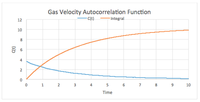
TASK: In the theoretical section at the beginning, the equation for the evolution of the position of a 1D harmonic oscillator as a function of time was given. Using this, evaluate the normalised velocity autocorrelation function for a 1D harmonic oscillator (it is analytic!):

$C (τ) = \frac{\int_{- \infty}^{\infty} v (t) v (t + τ) d t}{\int_{- \infty}^{\infty} v^{2} (t) d t}$

On the same graph, with x range 0 to 500, plot $C (τ)$ with $ω = 1 / 2 π$ and the VACFs from your liquid and solid simulations. What do the minima in the VACFs for the liquid and solid system represent? Discuss the origin of the differences between the liquid and solid VACFs. The harmonic oscillator VACF is very different to the Lennard Jones solid and liquid. Why is this? Attach a copy of your plot to your writeup.

The liquid simulation shows a minima around 0.2, this is due to a liquid particle- particle collision, causing both particles to reverse in direction. This is why the correlated velocity is negative. The velocity generator in the script generates the velocity randomly, and hence once the liquid particles have lost that initial velocity after the collision and started moving around according to the laws of Brownian motion, then the correlation decays to zero. Hence a particle’s velocity at time 0.4 is completely unrelated to its velocity at the beginning of time. The intermolecular forces are strong in high density systems such as liquids and solids. The velocity correlation quickly decays to zero because of the destructive intermolecular forces that the liquid particles experience. The difference for liquids is that liquids do not have fixed atomic positions for each particle, like a solid does, so the particles will diffuse very quickly after initiating the simulation. What is observed on the graph is similar to a very damped oscillation, (the minima in the beginning of the graph) where two particles collide and rebound in opposite directions. (The rebound is shown when the graph on the y-axis becomes negative, which is when the velocity change direction.

NJ: The VACF is only measured over the equilibrium part of the simulation, not the beginning. The first liquid minimum is due to collision with the "solvent cage".

The solid simulation shows a longer decay than the liquid. It also has a very large negative minima in the beginning of the simulation. This is because the randomly generated velocity gives the particles a lot of kinetic energy, causing collision to happen as they are all generated in a high density lattice structure. Under such an environment collisions are much more likely to happen, which is why the minima is a much larger value than in the liquid. The solid has a longer decay because due to the ordered structure of a solid, particles can find an energetically stable position which balances attractive and repulsive forces. The motion in the solid is all due to oscillations, whereby the particle oscillates in different directions from its equilibrium position. Hence the function is similar to that of a damped harmonic oscillator. However the oscillation does not correlate to the magnitude of the VACF. The reason for the decay time is particles in a solid still experience destructive forces which will disrupts with the initial force created by the velocity, until finally the velocity is uncorrelated.

NJ: Again, good explanation, but this isn't data from the initial part of the simulation. It's averaged over many "initial" velocities. Don't call the forces destructive, it's not meaningful here. You can say that the interatomic collisions causes the atomic velocities to become decorrelated.

The harmonic oscillator never decays. The harmonic oscillator is isolated and does not interact with other atoms. The harmonic oscillator does not experience destructive forces like the Lennard Jones potential or the attractive and repulsive intermolecular forces or friction. The harmonic oscillator undergoes simple harmonic motion with a constant amplitude and a constant frequency.The change in VACF observed in the harmonic oscillator is the natural change in velocity observed when the oscillator finishes its swing at a high potential energy with no kinetic energy and falls back down accelerating to full velocity, at which it crosses the x-axis.

NJ: Excellent

Shown in Fig.26 below, the graph for VACF shows a system where the intermolecular forces are very small yet not negligible. These gas molecules will under go a very slow decay, as the destructive intermolecular forces slowly interfere until the velocity is no longer correlated.

TASK: Use the trapezium rule to approximate the integral under the velocity autocorrelation function for the solid, liquid, and gas, and use these values to estimate $D$ in each case. You should make a plot of the running integral in each case. Are they as you expect? Repeat this procedure for the VACF data that you were given from the one million atom simulations. What do you think is the largest source of error in your estimates of D from the VACF?

D from VACF	Solid	Liquid	Gas
Simulated Data	$0.132$	$0.157$	$3.201$
1 Million Atom Data	$0.04$	$0.0347$	$3.26$

The integral graphs compared to the 1 Million Atom simulation are very similar.

These values of the diffusion coefficient do not agree with the diffusion coefficients calculated above for MSD.

The largest source of error in estimates of D from the VACF is from the fact the the function doesn't take into account the position of the atoms. The value of D is calculated by multiplying the integral of the VACF function with a factor of one third. The graph only takes into account the correlation of the velocity and doesn't not take into account the initial position and the final position of the atom, which is why in solids the values for diffusion coefficient have increased by several magnitudes compared to the MSD values simply because VACF integral takes all the oscillation and vibrational energy into account, without considering that this may just be molecular oscillation in equilibrium position and that the net displacement of the atom is close to zero. This is why the values of D from the VACF is much larger. On the other hand, the liquid and gas simulations all have larger diffusion coefficient. Although the error is less observed in their case, since liquids and gas properties allow the particles to move around, hence the VACF can estimate the diffusion of the particles to a large extent, but it will still take into account the particle's vibrational energy in its integral.

NJ: Incorrect. When using the VACF approach, the positions aren't relevant - only the velocities. Did you integrate the absolute VACF? Your values seems a bit large. You have to integrate the VACF including the negative contributions.

Another source of error in calculating the values of D is the trapezium rule. The trapezium rule divides the area under the curve into various small trapeziums and calculate the sum of their area. The accuracy of the results completely depend on how large the x values used are. For instance in the current graphs, the trapezium rule is using the timestep value for incremental increases, however this can be modified to have smaller increments and hence increasing the accuracy.

References

Ref. 1 Phillips, Anthony. 'A Brief Note: Why Fcc Has 12 Nearest Neighbours'. Ph.qmul.ac.uk. N.p., 2015. Web. 20 Nov. 2015.

Ref.2 ifmpan,. 'FCC And Its Neighbours'. N.p., 2015. Web. 20 Nov. 2015.