Talk:Mod:ia2514 cmp

JC: General comments: Good understanding of the steps in the experiment and report is well written and laid out. Some of the explanations could be expanded to explain or speculate on why you get some of the trends that you see.

Introduction to the Ising model

This experiment involved conducting a Monte Carlo simulation on square Ising lattices using Python in order to compute the average energies and magnetisations. The obtained data was plotted and compared for various lattice sizes and the energy and energy squared values allowed for the calculation of the heat capacity. The data was also compared with C++ data from longer simulations which was then used to determine the Curie temperature for the 2D infinite lattice. The obtained value was in agreement with the analytical solution and the lack of precision was attributed to employing the Monte Carlo sampling method, to the contribution of the relaxation energy values to the averaging and the noise in the heat capacity data.

Introduction to the Ising model

In this part of the experiment, the minimum energy, multiplicity and entropy of the Ising model was determined and values were calculated for particular cases.

Task 1

Show that the lowest possible energy for the Ising model is $E = - D N J$ , where $D$ is the number of dimensions and $N$ is the total number of spins. What is the multiplicity of this state? Calculate its entropy.

The interaction energy is $E = - \frac{1}{2} J \sum_{i}^{N} \sum_{j \in n e i g h b o u r s (i)} s_{i} s_{j}$ .

The lowest possible energy for the Ising model is obtained when all the spins have the same value (either +1 or -1) $\Rightarrow s_{i} s_{j} = 1, \forall i, j$ $\Rightarrow E_{m i n} = - \frac{1}{2} J \sum_{i}^{N} \sum_{j \in n e i g h b o u r s (i)} 1$

Each spin has $2 D$ neighbours (2 in each direction, where $D$ is the number of dimensions) $\Rightarrow E_{m i n} = - \frac{1}{2} \times J \times N \times 2 D \Leftrightarrow E_{m i n} = - D N J$

The multiplicity of this state is $\frac{N!}{\sum_{i} n_{i}!} = \frac{N!}{N!} = 1$ since all the spins have the same orientation ( $n_{1} = N$ ).

The entropy can be calculated using Boltzmann's equation: $S = k_{B} \ln W$ where $W$ is the number of microstates. Since there is only one configuration for each of the two different states in which all the spins are equal (all spins either -1 or +1), $W = 1$ and the entropy is $S = 0$ .

JC: Good clear derivation of the minimum energy. What is the n_i in the denominator of the multiplicity - the numerator should be the number of particles (lattice sites in this case) and the denominator the number which are distinguishable (N! in this case, since all lattice sites are distinguishable by their coordinates on the lattice).

Task 2

Imagine that the system is in the lowest energy configuration. To move to a different state, one of the spins must spontaneously change direction ("flip"). What is the change in energy if this happens ( $D = 3, N = 1000$ )? How much entropy does the system gain by doing so?

If starting from the state with the lowest energy (all spins equal) one of the spins changes directions, let the energy of the new system be $E^{'} = - \frac{1}{2} J \sum_{i}^{N} \sum_{j \in n e i g h b o u r s (i)} s_{i} s_{j}$ .

There are $2 D N$ neighbour interactions in total (double counted; 2 interactions in each of the $D$ directions for each of the $N$ spins).

Out of these, $4 D$ interactions include the flipped spin and have the product of the neighbouring spins $s_{i} s_{j} = - 1$ , while the rest of $2 D N - 4 D$ interactions have $s_{i} s_{j} = 1$ .

The interaction energy is therefore $E^{'} = - \frac{1}{2} J \times 2 D (N - 2) + \frac{1}{2} J \times 4 D \Rightarrow E^{'} = - D (N - 4) J$ .

Since the minimum energy is $E_{m i n} = - D N J$ , the energy difference is $Δ E = E^{'} - E_{m i n} = 4 D J$ .

For the new system, with one spin flipped, $W^{'} = N$ and the entropy is $S^{'} = k_{B} \ln N$ .

For such a system with $D = 3$ and $N = 1000$ , the change in energy when a spin flips is $Δ E = 12 J$ and the gain in entropy is $Δ S = k_{B} \ln 1000 = 9.53 \times 1 0^{23} J K^{- 1}$ .

JC: Correct.

Task 3

Calculate the magnetisation of the 1D and 2D lattices in figure 1. What magnetisation would you expect to observe for an Ising lattice with $D = 3, N = 1000$ at absolute zero?

The magnetisation of a system is $M = \sum_{i} s_{i}$ . For the 1D lattice in figure 1, $M_{1 D} = 1$ and for the 2D lattice, $M_{2 D} = 1$ .

At absolute zero, the system is expected to have minimum energy, since no thermal energy is available to overcome the interaction energy between spins of opposite orientations and therefore all the spins are aligned (either +1 or -1). The magnetisation in this case is either $M_{0 K} = N = 1000$ or $M_{0 K} = - N = - 1000$ .

JC: Correct.

Calculating the energy and magnetisation

In the second part of the experiment, the energy() and magnetisation() methods of the IsingLattice class were completed to determine the energy and magnetisation of a two-dimensional Ising lattice and the calculated results were as expected.

Task 4

Complete the functions energy() and magnetisation(), which should return the energy of the lattice and the total magnetisation, respectively. In the energy() function you may assume that $J = 1.0$ at all times (in fact, we are working in reduced units in which $J = k_{B}$ , but there will be more information about this in later sections). Do not worry about the efficiency of the code at the moment — we will address the speed in a later part of the experiment.

In order to account for the periodic boundary condition, two variables are defined for the row number of the neighbour below and the column number of the neighbour to the right of the current spin. In the case of the spins on the last row or column of the lattice, these variables take the value 0.

def energy(self):
   
    "Returns the total energy of the current lattice configuration."
   
    energy = 0.0
    J = 1

    for i in range(0,self.n_rows):
        for j in range(0,self.n_cols):
           
            if i < self.n_rows-1: #row number of neighbour below if the current spin is not on the last row of the lattice
                down_r = i+1
            else: down_r=0 #row number of neighbour below if the current spin is on the last row of the lattice
           
            if j < self.n_cols-1: #column number of neighbour to the right if the current spin is not on the last column of the lattice
                right_c = j+1
            else: right_c = 0 #column number of neighbour to the right if the current spin is on the last column of the lattice
           
            energy = energy - 1/2*J*self.lattice[i,j]*(self.lattice[i-1,j] + self.lattice[down_r,j] + self.lattice[i,j-1] + self.lattice[i,right_c])
           
    return energy

def magnetisation(self):

    "Returns the total magnetisation of the current lattice configuration."

    magnetisation = 0.0

    for i in range(0,self.n_rows):
        for j in range(0,self.n_cols):

            magnetisation = magnetisation + self.lattice[i,j]

    return magnetisation

JC: Code looks good and well commented.

Task 5

Run the ILcheck.py script from the IPython Qt console using the command

%run ILcheck.py

The displayed window has a series of control buttons in the bottom left, one of which will allow you to export the figure as a PNG image. Save an image of the ILcheck.py output, and include it in your report.

As shown in figure 1, the calculated values for the energy and magnetisation match the expected values.

Introduction to Monte Carlo simulation

Since analysing all the possible states of a system would require extensive computational time (of the order of trillions of years for 100 spins), the Monte Carlo sampling method was implemented. The montecarlostep() and statistics() methods were completed to run one Monte Carlo step and calculate and return the averaged energies and magnetisations, respectively, and the simulation was run with the energy and magnetisation graphs displayed in real time.

Task 6

How many configurations are available to a system with 100 spins? To evaluate these expressions, we have to calculate the energy and magnetisation for each of these configurations, then perform the sum. Let's be very, very, generous, and say that we can analyse $1 \times 1 0^{9}$ configurations per second with our computer. How long will it take to evaluate a single value of ${⟨ M ⟩}_{T}$ ?

Since each of the 100 spins can have 2 different orientations, there are $2^{100} \approx 1.27 \times 1 0^{30}$ possible configurations for this system. The time taken to evaluate ${⟨ M ⟩}_{T}$ (i.e. the time taken to analyse $2^{100}$ configurations at a speed of $1 \times 1 0^{9}$ configurations per second) is $\frac{2^{100}}{1 0^{9}} \approx \frac{1.27 \times 1 0^{30}}{1 0^{9}} = 1.27 \times 1 0^{21} s = 4.03 \times 1 0^{13} y e a r s$ .

JC: Correct.

Task 7

Implement a single cycle of the above algorithm in the montecarlocycle(T) function. This function should return the energy of your lattice and the magnetisation at the end of the cycle. You may assume that the energy returned by your energy() function is in units of $k_{B}$ ! Complete the statistics() function. This should return the following quantities whenever it is called: $< E >, < E^{2} >, < M >, < M^{2} >$ , and the number of Monte Carlo steps that have elapsed.

def montecarlostep(self, T):
    
    "Runs a single Monte Carlo step and returns the energy and magnetisation of the system."

    energy = self.energy()

    #selecting the coordinates of the random spin
    random_i = np.random.choice(range(0, self.n_rows))
    random_j = np.random.choice(range(0, self.n_cols))
   
    new_il=copy.deepcopy(self)
   
    new_il.lattice[random_i,random_j]=-new_il.lattice[random_i,random_j] #a random spin is flipped
   
    en_difference = new_il.energy() - energy
    if en_difference<0:
        self.lattice=new_il.lattice
        energy=self.energy()
    else:
        #choosing a random number in the range [0,1)
        random_number = np.random.random()
        if random_number<=e**(-en_difference/T):
            self.lattice=new_il.lattice
            energy=self.energy()
        else:
            pass
    self.statistics()
    
    return self.energy(), self.magnetisation()

def statistics(self):

    "Calculates and returns the values for the averages of E, E*E, M, M*M, and the number of Monte Carlo steps that have been performed."

    self.n_cycles += 1
    self.E=self.E+self.energy()
    self.E2=self.E2+self.energy()**2
    self.M=self.M+self.magnetisation()
    self.M2=self.M2+self.magnetisation()**2
   
    return self.E/self.n_cycles,self.E2/self.n_cycles,self.M/self.n_cycles,self.M2/self.n_cycles,self.n_cycles

JC: Code looks correct.

Task 8

If $T < T_{C}$ , do you expect a spontaneous magnetisation (i.e. do you expect $⟨ M ⟩ \neq 0$ )? When the state of the simulation appears to stop changing (when you have reached an equilibrium state), use the controls to export the output to PNG and attach this to your report. You should also include the output from your statistics() function.

At $T < T_{C}$ spontaneous magnetisation is expected (i.e. $⟨ M ⟩ \neq 0$ ) for a ferromagnet. However, the magnetisation is expected to approach zero as the temperature increases towards $T_{C}$ , according to a power law: $M (T) \sim (T_{C} - T)^{β}$ where $β$ is positive.^[1]

**Figure 2.** ILanim.py frame after the system has reached equilibrium

**Figure 3.** statistics() output after the system has reached equilibrium

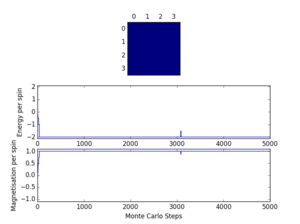
The output in figure 3 suggests that the calculated average values are not an accurate representation of the system at equilibrium due to the relaxation period.

Accelerating the code

In this section of the experiment the code was accelerated by replacing the two for loops used in order to access all the matrix elements with a single linear calculation.

Task 9

Use the script ILtimetrial.py to record how long your current version of IsingLattice.py takes to perform 2000 Monte Carlo steps. This will vary, depending on what else the computer happens to be doing, so perform repeats and report the error in your average!

**Table 1.** Time taken to perform 2000 Monte Carlo steps (current version of IsingLattice.py)
Time/s	Average time/s
17.29	17.23 $\pm$ 0.04
17.21
17.19
17.22
17.23

The time taken to perform 2000 Monte Carlo steps using the current version of IsingLattice.py was recorded 5 times, the uncertainty in the average value arising mainly due to the computer performing other tasks at the same time.

Task 10

Look at the documentation for the NumPy sum function. You should be able to modify your magnetisation() function so that it uses this to evaluate M. The energy is a little trickier. Familiarise yourself with the NumPy roll and multiply functions, and use these to replace your energy double loop (you will need to call roll and multiply twice!).

The roll function was used to shift the last row and last column, respectively to the front of the lattice. The two new lattices obtained this way were each multiplied with the original one and the sum of all the elements of the matrices resulting from the multiplication was used in order to calculate the energy.

def energy(self):

    "Returns the total energy of the current lattice configuration."

    J = 1

    energy = - J*(np.sum(np.multiply(self.lattice,np.roll(self.lattice,1,axis=1)))+np.sum(np.multiply(self.lattice,np.roll(self.lattice,1,axis=0))))

    return energy

def magnetisation(self):

    "Returns the total magnetisation of the current lattice configuration."

    magnetisation = np.sum(self.lattice)
    
    return magnetisation

JC: Good use of roll and multiply, well noticed that you only need to use roll twice if you remove the factor of 1/2 for double counting.

Task 11

Use the script ILtimetrial.py to record how long your new version of IsingLattice.py takes to perform 2000 Monte Carlo steps. This will vary, depending on what else the computer happens to be doing, so perform repeats and report the error in your average!

**Table 2.** Time taken to perform 2000 Monte Carlo steps (new version of IsingLattice.py)
Time/s	Average time/s
0.35	0.35 $\pm$ 0.00
0.35
0.35
0.34
0.35

The new version of IsingLattice.py runs almost 50 times faster than the previous one.

JC: Good.

The effect of temperature

Simulations were run for various lattice sizes at different temperatures and based on the number of steps required to reach equilibrium the first 200,000 cycles were excluded from the averaging. This resulted in small error bars in the subsequent energy and magnetisation versus temperature plots.

Task 12

The script ILfinalframe.py runs for a given number of cycles at a given temperature, then plots a depiction of the final lattice state as well as graphs of the energy and magnetisation as a function of cycle number. This is much quicker than animating every frame! Experiment with different temperature and lattice sizes. How many cycles are typically needed for the system to go from its random starting position to the equilibrium state? Modify your statistics() and montecarlostep() functions so that the first N cycles of the simulation are ignored when calculating the averages. You should state in your report what period you chose to ignore, and include graphs from ILfinalframe.py to illustrate your motivation in choosing this figure.

4x4 lattice at temperature T=1	8x8 lattice at temperature T=1	16x16 lattice at temperature T=1
32x32 lattice at temperature T=1	32x32 lattice at temperature T=2	32x32 lattice at temperature T=3
Figure 4. ILfinalframe.py plots for various lattice sizes and temperatures

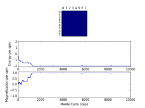
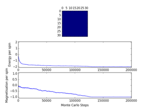
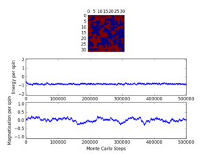
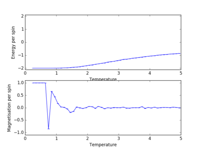
The simulation was run for 2x2, 4x4, 8x8, 16x16 and 32x32 lattices at temperatures from 0.25 to 5.00 and some of the resulting graphs are presented in figure 4. For a given temperature, the number of cycles needed to equilibrate increases with lattice size. The number of cycles needed to reach equilibrium is expected to increase as the temperature approaches $T_{C}$ from below since the magnetisation drops to zero as the temperature increases towards the Curie temperature ^[1]. Above the Curie Temperature, starting from a random lattice, the systems reach equilibrium faster since no spontaneous magnetisation is expected. Therefore, the largest lattice at a temperature just below the Curie Temperature requires the most cycles to equilibrate.

JC: Good reasoning and good choice of length of equilibration period.

As observed in figure 4, the 32x32 lattice at T=2 reached equilibrium after about 180000 steps, so the first $N = 200000$ cycles were further chosen to be ignored when calculating the average (N was added as a class attribute):

def montecarlostep(self, T):
    
    "Runs a single Monte Carlo step and returns the energy and magnetisation of the system."

    energy = self.energy()

    #selecting the coordinates of the random spin
    random_i = np.random.choice(range(0, self.n_rows))
    random_j = np.random.choice(range(0, self.n_cols))
   
    new_il=copy.deepcopy(self)
   
    new_il.lattice[random_i,random_j]=-new_il.lattice[random_i,random_j] #a random spin is flipped
   
    en_difference = new_il.energy() - energy
    if en_difference<0:
        self.lattice=new_il.lattice
        energy=self.energy()
    else:
        #choosing a random number in the range [0,1)
        random_number = np.random.random()
        if random_number<=e**(-en_difference/T):
            self.lattice=new_il.lattice
            energy=self.energy()
        else:
            pass

    self.n_cycles += 1

    if self.n_cycles>self.N: 
        self.statistics()
    
    return self.energy(), self.magnetisation()

def statistics(self):

    "Calculates and returns the values for the averages of E, E*E, M, M*M, and the number of Monte Carlo steps that have been performed."

    self.E=self.E+self.energy()
    self.E2=self.E2+self.energy()**2
    self.M=self.M+self.magnetisation()
    self.M2=self.M2+self.magnetisation()**2
   
    return self.E/(self.n_cycles-self.N),self.E2/(self.n_cycles-self.N),self.M/(self.n_cycles-self.N),self.M2/(self.n_cycles-self.N),self.n_cycles

Task 13

Use ILtemperaturerange.py to plot the average energy and magnetisation for each temperature, with error bars, for an $8 \times 8$ lattice. Use your initution and results from the script ILfinalframe.py to estimate how many cycles each simulation should be. The temperature range 0.25 to 5.0 is sufficient. Use as many temperature points as you feel necessary to illustrate the trend, but do not use a temperature spacing larger than 0.5. T NumPy function savetxt() stores your array of output data on disk — you will need it later. Save the file as 8x8.dat so that you know which lattice size it came from.

from IsingLattice import *
from matplotlib import pylab as pl
import numpy as np

n_rows = 8
n_cols = 8
il = IsingLattice(n_rows, n_cols)
il.lattice = np.ones((n_rows, n_cols))
spins = n_rows*n_cols
runtime = 300000
times = range(runtime)
temps = np.arange(0.25, 5.0, 0.1)
energies = []
magnetisations = []
energies_error=[]
magnetisations_error=[]
energysq = []
magnetisationsq = []
for t in temps:
    en_array=[]
    magn_array=[]
    for i in times:
        if i % 100 == 0:
            print(t, i)
        energy, magnetisation = il.montecarlostep(t)
        en_array.append(energy)    #array of all the energies for a certain temperature
        magn_array.append(magnetisation)    #array of all the magnetisations for a certain temperature
    en_error=np.std(en_array,ddof=1)/len(en_array)**0.5    #energy error for the current temperature
    magn_error=np.std(magn_array,ddof=1)/len(magn_array)**0.5    #magnetisation error for the current temperature
    energies_error.append(en_error)    #array of all the energy errors
    magnetisations_error.append(magn_error)    #array of all the magnetisation errors

    aveE, aveE2, aveM, aveM2, n_cycles = il.statistics()
    energies.append(aveE)
    energysq.append(aveE2)
    magnetisations.append(aveM)
    magnetisationsq.append(aveM2)
    #reset the IL object for the next cycle
    il.E = 0.0
    il.E2 = 0.0
    il.M = 0.0
    il.M2 = 0.0
    il.n_cycles = 0
fig = pl.figure()
enerax = fig.add_subplot(2,1,1)
enerax.set_ylabel("Energy per spin")
enerax.set_xlabel("Temperature")
enerax.set_ylim([-2.1, 2.1])
magax = fig.add_subplot(2,1,2)
magax.set_ylabel("Magnetisation per spin")
magax.set_xlabel("Temperature")
magax.set_ylim([-1.1, 1.1])
enerax.errorbar(temps, np.array(energies)/spins,yerr=energies_error)    #errorbar instead of plot to add errorbars
magax.errorbar(temps, np.array(magnetisations)/spins,yerr=magnetisations_error)
pl.show()

final_data = np.column_stack((temps, energies, energysq, magnetisations, magnetisationsq))
np.savetxt("8x8.dat", final_data)

The simulation was run for a total of 300000 steps (out of which the first 200000 cycles were excluded from the averaging) and for temperatures between 0.25 and 5.00 in steps of 0.1.

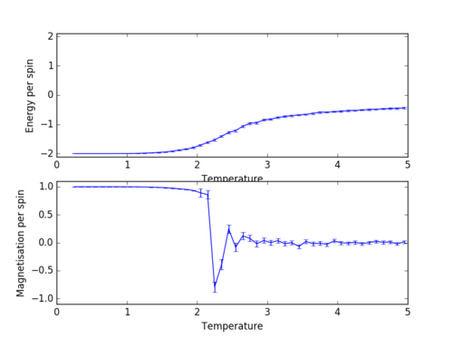
As seen in figure 5, there is an increase in energy around the Curie temperature and a sharp decrease in magnetisation followed by a gradually damped oscillation around the zero value. As expected, the largest errors are exhibited in the oscillation area of the magnetisation graph.

JC: Good.

The effect of system size

In this part of the experiment energy and magnetisation versus temperature graphs were plotted and compared for various lattice sizes.

Task 14

Repeat the final task of the previous section for the following lattice sizes: 2x2, 4x4, 8x8, 16x16, 32x32. Make sure that you name each datafile that your produce after the corresponding lattice size! Write a Python script to make a plot showing the energy per spin versus temperature for each of your lattice sizes. Hint: the NumPy loadtxt function is the reverse of the savetxt function, and can be used to read your previously saved files into the script. Repeat this for the magnetisation. As before, use the plot controls to save your a PNG image of your plot and attach this to the report. How big a lattice do you think is big enough to capture the long range fluctuations?

2x2 lattice	4x4 lattice
16x16 lattice	32x32 lattice
Figure 6. Energy per spin and magnetisation per spin as functions of temperature for various lattice sizes

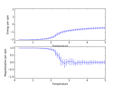
A similar behaviour to the case of the 8x8 lattice (figure 5) is observed for the 2x2, 4x4, 16x16 and 32x32 lattices (figure 6). The output .dat files were used to plot the energy and magnetisation per spin for all the different lattice sizes:

from matplotlib import pylab as pl
import numpy as np


data2=np.loadtxt('2x2.dat')
data4=np.loadtxt('4x4.dat')
data8=np.loadtxt('8x8.dat')
data16=np.loadtxt('16x16.dat')
data32=np.loadtxt('32x32.dat')

en2=data2[:,1]
en4=data4[:,1]
en8=data8[:,1]
en16=data16[:,1]
en32=data32[:,1]

magn2=data2[:,3]
magn4=data4[:,3]
magn8=data8[:,3]
magn16=data16[:,3]
magn32=data32[:,3]

fig = pl.figure()
pl.title("Energy and magnetisation per spin versus temperature for various lattice sizes")

enerax = fig.add_subplot(2,1,1)
enerax.set_ylabel("Energy per spin")
enerax.set_xlabel("Temperature")
enerax.set_ylim([-2.1, 2.1])
magax = fig.add_subplot(2,1,2)
magax.set_ylabel("Magnetisation per spin")
magax.set_xlabel("Temperature")
magax.set_ylim([-1.1, 1.1])

enerax.plot(data2[:,0], en2/(2*2), label="2x2")
enerax.plot(data4[:,0], en4/(4*4), label="4x4")
enerax.plot(data8[:,0], en8/(8*8), label="8x8")
enerax.plot(data16[:,0], en16/(16*16), label="16x16")
enerax.plot(data32[:,0], en32/(32*32), label="32x32")
enerax.legend(loc=2,title="Lattice size",fontsize="10")

magax.plot(data2[:,0], magn2/(2*2), label="2x2")
magax.plot(data4[:,0], magn4/(4*4), label="4x4")
magax.plot(data8[:,0], magn8/(8*8), label="8x8")
magax.plot(data16[:,0], magn16/(16*16), label="16x16")
magax.plot(data32[:,0], magn32/(32*32), label="32x32")
magax.legend(loc="best",title="Lattice size",fontsize="10")

pl.show()

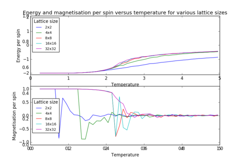
**Figure 7.** Energy and magnetisation per spin versus temperature for various lattice sizes

As shown in figure 7, the sharp decrease in magnetisation occurs at lower temperatures for the smaller lattices and the steepness of the energy versus temperature curve decreases with decreasing lattice size, the graph becoming almost linear for the 2x2 lattice. Long range fluctuations are visible for lattices between 2x2 and 16x16 which could suggest that in the case of larger lattices (32x32), the fluctuations have a higher frequency and the system equilibrates over a narrow temperature range which would require a temperature spacing smaller than 0.1 (i.e. more data points) in order to be observed.

JC: How can you tell that long range fluctuations are present from these graphs? Long range fluctuations become most significant close to Tc. If a particular lattice size captures long range fluctuations the energy vs temperature curve should converge with the curves for larger systems.

Determining the heat capacity

An expression for the heat capacity as a function of the energy variance and temperature was derived and then used to plot heat capacity versus temperature graphs for various lattice sizes.

Task 15

By definition,

$C = \frac{\partial ⟨ E ⟩}{\partial T}$

From this, show that

$C = \frac{V a r [E]}{k_{B} T^{2}}$

(Where $V a r [E]$ is the variance in $E$ .)

${⟨ E ⟩}_{T} = \frac{1}{Z} \sum_{α} E (α) \exp {- \frac{E (α)}{k_{B} T}}$ where the partition function $Z = \sum_{α} \exp {- \frac{E (α)}{k_{B} T}}$ .

Introducing the notation $β = \frac{1}{k_{B} T}$ , ${⟨ E ⟩}_{T}$ can be rewritten as ${⟨ E ⟩}_{T} = - \frac{1}{Z} \frac{\partial Z}{\partial β}$ and therefore

${⟨ E ⟩}_{T}^{2} = \frac{1}{Z^{2}} {(\frac{\partial Z}{\partial β})}^{2}$ (1)

since $\frac{\partial Z}{\partial β} = \frac{\partial \sum_{α} \exp {- β E (α)}}{\partial β} = - \sum_{α} E (α) \exp {- β E (α)}$ .

Analogously to the expression of ${⟨ E ⟩}_{T}$ , ${⟨ E^{2} ⟩}_{T} = \frac{1}{Z} \sum_{α} E {(α)}^{2} \exp {- \frac{E (α)}{k_{B} T}}$ .

Since $\frac{\partial^{2} Z}{\partial β^{2}} = \frac{\partial}{\partial β} (- \sum_{α} E (α) \exp {- β E (α)}) = \sum_{α} E {(α)}^{2} \exp {- \frac{E (α)}{k_{B} T}}$ it follows that

${⟨ E^{2} ⟩}_{T} = \frac{1}{Z} \frac{\partial^{2} Z}{\partial β^{2}}$ (2)

By definition, $C = \frac{\partial ⟨ E ⟩}{\partial T}$ and from the expression for ${⟨ E ⟩}_{T}$ it follows that:

$\begin{aligned} C & = \frac{\partial}{\partial T} (- \frac{1}{Z} \frac{\partial Z}{\partial β}) \\ = \frac{\partial (- \frac{1}{Z})}{\partial T} \frac{\partial Z}{\partial β} - \frac{1}{Z} \frac{\partial}{\partial T} (\frac{\partial Z}{\partial β}) \\ = \frac{\partial (- \frac{1}{Z})}{\partial β} \frac{\partial β}{\partial T} \frac{\partial Z}{\partial β} - \frac{1}{Z} \frac{\partial (\frac{\partial Z}{\partial β})}{\partial β} \frac{\partial β}{\partial T} \\ = - \frac{1}{k_{B} T^{2}} \frac{\partial (- \frac{1}{Z})}{\partial Z} \frac{\partial Z}{\partial β} \frac{\partial Z}{\partial β} + \frac{1}{Z k_{B} T^{2}} \frac{\partial^{2} Z}{\partial β^{2}} \\ = \frac{1}{k_{B} T^{2}} (- \frac{1}{Z^{2}} {(\frac{\partial Z}{\partial β})}^{2} + \frac{1}{Z} \frac{\partial^{2} Z}{\partial β^{2}}) \end{aligned}$

From (1) and (2) it can be seen that $C = \frac{1}{k_{B} T^{2}} ({⟨ E^{2} ⟩}_{T} - {⟨ E ⟩}_{T}^{2})$ and given that $V a r [E] = {⟨ E^{2} ⟩}_{T} - {⟨ E ⟩}_{T}^{2}$ , the conclusion follows.

JC: Good derivation.

Task 16

Write a Python script to make a plot showing the heat capacity versus temperature for each of your lattice sizes from the previous section. You may need to do some research to recall the connection between the variance of a variable, $V a r [X]$ , the mean of its square $⟨ X^{2} ⟩$ , and its squared mean ${⟨ X ⟩}^{2}$ . You may find that the data around the peak is very noisy — this is normal, and is a result of being in the critical region. As before, use the plot controls to save your a PNG image of your plot and attach this to the report.

from matplotlib import pylab as pl
import numpy as np


data2=np.loadtxt('2x2.dat')
data4=np.loadtxt('4x4.dat')
data8=np.loadtxt('8x8.dat')
data16=np.loadtxt('16x16.dat')
data32=np.loadtxt('32x32.dat')

#extract temperature values (same for all lattice sizes)
temps=data2[:,0]

#extract energy values
en2=data2[:,1]
en4=data4[:,1]
en8=data8[:,1]
en16=data16[:,1]
en32=data32[:,1]

#extract energy squared values
ensq2=data2[:,2]
ensq4=data4[:,2]
ensq8=data8[:,2]
ensq16=data16[:,2]
ensq32=data32[:,2]

#extract magnetisation values
magn2=data2[:,3]
magn4=data4[:,3]
magn8=data8[:,3]
magn16=data16[:,3]
magn32=data32[:,3]

#extract magnetisation squared values
magnsq2=data2[:,4]
magnsq4=data4[:,4]
magnsq8=data8[:,4]
magnsq16=data16[:,4]
magnsq32=data32[:,4]

pl.ylabel("Heat capacity")
pl.xlabel("Temperature")

pl.plot(temps,(ensq2-en2**2)/temps**2,label="2x2")
pl.plot(temps,(ensq4-en4**2)/temps**2,label="4x4")
pl.plot(temps,(ensq8-en8**2)/temps**2,label="8x8")
pl.plot(temps,(ensq16-en16**2)/temps**2,label="16x16")
pl.plot(temps,(ensq32-en32**2)/temps**2,label="32x32")
pl.title("Heat capactiy versus temperature for various lattice sizes")
pl.legend(loc="best",title="Lattice size",fontsize="10")

pl.show()

**Figure 8.** Heat capacity versus temperature for various lattice sizes

As shown in figure 8, the heat capacity at a given temperature increases with lattice size and the graph of the heat capacity against temperature is more sharply peaked the larger the lattice.

JC: Does this trend make sense?

Locating the Curie temperature

The data obtained from the Python algorithm was compared with C++ data from longer simulations. The heat capacity data was fitted to a polynomial in order to determine the peak values more accurately which were then used to calculate the Curie temperature for an infinite 2D Ising lattice.

Task 17

A C++ program has been used to run some much longer simulations than would be possible on the college computers in Python. You can view its source code here if you are interested. Each file contains six columns: $T, E, E^{2}, M, M^{2}, C$ (the final five quantities are per spin), and you can read them with the NumPy loadtxt function as before. For each lattice size, plot the C++ data against your data. For one lattice size, save a PNG of this comparison and add it to your report — add a legend to the graph to label which is which. To do this, you will need to pass the label="..." keyword to the plot function, then call the legend() function of the axis object (documentation here).

In the following script, the user can input what quantity to be compared between the Python and the C++ data and for which lattice size:

from matplotlib import pylab as pl
import numpy as np

lattice_size=input('Lattice size: ')
to_plot=input('Plot (energy - 1; energy squared - 2; magnetisation - 3; magnetisation squared - 4; heat capacity - 5): ')

#Python data
data2=np.loadtxt('2x2.dat')
data4=np.loadtxt('4x4.dat')
data8=np.loadtxt('8x8.dat')
data16=np.loadtxt('16x16.dat')
data32=np.loadtxt('32x32.dat')

#C++ data
c_data2=np.loadtxt('C++_data/2x2.dat')
c_data4=np.loadtxt('C++_data/4x4.dat')
c_data8=np.loadtxt('C++_data/8x8.dat')
c_data16=np.loadtxt('C++_data/16x16.dat')
c_data32=np.loadtxt('C++_data/32x32.dat')

temps=data2[:,0]

en2=data2[:,1]
en4=data4[:,1]
en8=data8[:,1]
en16=data16[:,1]
en32=data32[:,1]

c_en2=c_data2[:,1]
c_en4=c_data4[:,1]
c_en8=c_data8[:,1]
c_en16=c_data16[:,1]
c_en32=c_data32[:,1]

ensq2=data2[:,2]
ensq4=data4[:,2]
ensq8=data8[:,2]
ensq16=data16[:,2]
ensq32=data32[:,2]

c_ensq2=c_data2[:,2]
c_ensq4=c_data4[:,2]
c_ensq8=c_data8[:,2]
c_ensq16=c_data16[:,2]
c_ensq32=c_data32[:,2]

magn2=data2[:,3]
magn4=data4[:,3]
magn8=data8[:,3]
magn16=data16[:,3]
magn32=data32[:,3]

c_magn2=c_data2[:,3]
c_magn4=c_data4[:,3]
c_magn8=c_data8[:,3]
c_magn16=c_data16[:,3]
c_magn32=c_data32[:,3]

magnsq2=data2[:,4]
magnsq4=data4[:,4]
magnsq8=data8[:,4]
magnsq16=data16[:,4]
magnsq32=data32[:,4]

c_magnsq2=c_data2[:,4]
c_magnsq4=c_data4[:,4]
c_magnsq8=c_data8[:,4]
c_magnsq16=c_data16[:,4]
c_magnsq32=c_data32[:,4]

c_heatcap2=c_data2[:,5]
c_heatcap4=c_data4[:,5]
c_heatcap8=c_data8[:,5]
c_heatcap16=c_data16[:,5]
c_heatcap32=c_data32[:,5]

if to_plot=='1':
    if lattice_size=='2':
        pl.ylabel("Energy per spin")
        pl.xlabel("Temperature")
        pl.plot(temps,en2/(2*2),label="Python")
        pl.plot(c_data2[:,0],c_en2,label="C++")
        pl.title("Python and C++ energy data comparison for a 2x2 lattice")
        pl.legend(loc="best",fontsize="10")
        pl.show()
    
    elif lattice_size=='4':
        pl.ylabel("Energy per spin")
        pl.xlabel("Temperature")
        pl.plot(temps,en4/(4*4),label="Python")
        pl.plot(c_data4[:,0],c_en4,label="C++")
        pl.title("Python and C++ energy data comparison for a 4x4 lattice")
        pl.legend(loc="best",fontsize="10")
        pl.show()
    
    
    elif lattice_size=='8':
        pl.ylabel("Energy per spin")
        pl.xlabel("Temperature")
        pl.plot(temps,en8/(8*8),label="Python")
        pl.plot(c_data8[:,0],c_en8,label="C++")
        pl.title("Python and C++ energy data comparison for a 8x8 lattice")
        pl.legend(loc="best",fontsize="10")
        pl.show()
    
    
    elif lattice_size=='16':
        pl.ylabel("Energy per spin")
        pl.xlabel("Temperature")
        pl.plot(temps,en16/(16*16),label="Python")
        pl.plot(c_data16[:,0],c_en16,label="C++")
        pl.title("Python and C++ energy data comparison for a 16x16 lattice")
        pl.legend(loc="best",fontsize="10")
        pl.show()
    
    
    elif lattice_size=='32':
        pl.ylabel("Energy per spin")
        pl.xlabel("Temperature")
        pl.plot(temps,en32/(32*32),label="Python")
        pl.plot(c_data32[:,0],c_en32,label="C++")
        pl.title("Python and C++ energy data comparison for a 32x32 lattice")
        pl.legend(loc="best",fontsize="10")
        pl.show()

elif to_plot=='2':
    if lattice_size=='2':
        pl.ylabel("Energy squared per spin")
        pl.xlabel("Temperature")
        pl.plot(temps,ensq2/(2*2)**2,label="Python")
        pl.plot(c_data2[:,0],c_ensq2,label="C++")
        pl.title("Python and C++ energy squared data comparison for a 2x2 lattice")
        pl.legend(loc="best",fontsize="10")
        pl.show()
    
    elif lattice_size=='4':
        pl.ylabel("Energy squared per spin")
        pl.xlabel("Temperature")
        pl.plot(temps,ensq4/(4*4)**2,label="Python")
        pl.plot(c_data4[:,0],c_ensq4,label="C++")
        pl.title("Python and C++ energy squared data comparison for a 4x4 lattice")
        pl.legend(loc="best",fontsize="10")
        pl.show()
    
    
    elif lattice_size=='8':
        pl.ylabel("Energy squared per spin")
        pl.xlabel("Temperature")
        pl.plot(temps,ensq8/(8*8)**2,label="Python")
        pl.plot(c_data8[:,0],c_ensq8,label="C++")
        pl.title("Python and C++ energy squared data comparison for a 8x8 lattice")
        pl.legend(loc="best",fontsize="10")
        pl.show()
    
    
    elif lattice_size=='16':
        pl.ylabel("Energy squared per spin")
        pl.xlabel("Temperature")
        pl.plot(temps,ensq16/(16*16)**2,label="Python")
        pl.plot(c_data16[:,0],c_ensq16,label="C++")
        pl.title("Python and C++ energy squared data comparison for a 16x16 lattice")
        pl.legend(loc="best",fontsize="10")
        pl.show()
    
    
    elif lattice_size=='32':
        pl.ylabel("Energy squared per spin")
        pl.xlabel("Temperature")
        pl.plot(temps,ensq32/(32*32)**2,label="Python")
        pl.plot(c_data32[:,0],c_ensq32,label="C++")
        pl.title("Python and C++ energy squared data comparison for a 32x32 lattice")
        pl.legend(loc="best",fontsize="10")
        pl.show()

elif to_plot=='3':
    if lattice_size=='2':
        pl.ylabel("Magnetisation per spin")
        pl.xlabel("Temperature")
        pl.plot(temps,magn2/(2*2),label="Python")
        pl.plot(c_data2[:,0],c_magn2,label="C++")
        pl.title("Python and C++ magnetisation data comparison for a 2x2 lattice")
        pl.legend(loc="best",fontsize="10")
        pl.show()
    
    elif lattice_size=='4':
        pl.ylabel("Magnetisation per spin")
        pl.xlabel("Temperature")
        pl.plot(temps,magn4/(4*4),label="Python")
        pl.plot(c_data4[:,0],c_magn4,label="C++")
        pl.title("Python and C++ magnetisation data comparison for a 4x4 lattice")
        pl.legend(loc="best",fontsize="10")
        pl.show()
    
    
    elif lattice_size=='8':
        pl.ylabel("Magnetisation per spin")
        pl.xlabel("Temperature")
        pl.plot(temps,magn8/(8*8),label="Python")
        pl.plot(c_data8[:,0],c_magn8,label="C++")
        pl.title("Python and C++ magnetisation data comparison for a 8x8 lattice")
        pl.legend(loc="best",fontsize="10")
        pl.show()
    
    
    elif lattice_size=='16':
        pl.ylabel("Magnetisation per spin")
        pl.xlabel("Temperature")
        pl.plot(temps,magn16/(16*16),label="Python")
        pl.plot(c_data16[:,0],c_magn16,label="C++")
        pl.title("Python and C++ magnetisation data comparison for a 16x16 lattice")
        pl.legend(loc="best",fontsize="10")
        pl.show()
    
    
    elif lattice_size=='32':
        pl.ylabel("Magnetisation per spin")
        pl.xlabel("Temperature")
        pl.plot(temps,magn32/(32*32),label="Python")
        pl.plot(c_data32[:,0],c_magn32,label="C++")
        pl.title("Python and C++ magnetisation data comparison for a 32x32 lattice")
        pl.legend(loc="best",fontsize="10")
        pl.show()

elif to_plot=='4':
    if lattice_size=='2':
        pl.ylabel("Magnetisation squared per spin")
        pl.xlabel("Temperature")
        pl.plot(temps,magnsq2/(2*2)**2,label="Python")
        pl.plot(c_data2[:,0],c_magnsq2,label="C++")
        pl.title("Python and C++ magnetisation squared data comparison for a 2x2 lattice")
        pl.legend(loc="best",fontsize="10")
        pl.show()
    
    elif lattice_size=='4':
        pl.ylabel("Magnetisation squared per spin")
        pl.xlabel("Temperature")
        pl.plot(temps,magnsq4/(4*4)**2,label="Python")
        pl.plot(c_data4[:,0],c_magnsq4,label="C++")
        pl.title("Python and C++ magnetisation squared data comparison for a 4x4 lattice")
        pl.legend(loc="best",fontsize="10")
        pl.show()
    
    
    elif lattice_size=='8':
        pl.ylabel("Magnetisation squared per spin")
        pl.xlabel("Temperature")
        pl.plot(temps,magnsq8/(8*8)**2,label="Python")
        pl.plot(c_data8[:,0],c_magnsq8,label="C++")
        pl.title("Python and C++ magnetisation squared data comparison for a 8x8 lattice")
        pl.legend(loc="best",fontsize="10")
        pl.show()
    
    
    elif lattice_size=='16':
        pl.ylabel("Magnetisation squared per spin")
        pl.xlabel("Temperature")
        pl.plot(temps,magnsq16/(16*16)**2,label="Python")
        pl.plot(c_data16[:,0],c_magnsq16,label="C++")
        pl.title("Python and C++ magnetisation squared data comparison for a 16x16 lattice")
        pl.legend(loc="best",fontsize="10")
        pl.show()
    
    
    elif lattice_size=='32':
        pl.ylabel("Magnetisation squared per spin")
        pl.xlabel("Temperature")
        pl.plot(temps,magnsq32/(32*32)**2,label="Python")
        pl.plot(c_data32[:,0],c_magnsq32,label="C++")
        pl.title("Python and C++ magnetisation squared data comparison for a 32x32 lattice")
        pl.legend(loc="best",fontsize="10")
        pl.show()        
        
elif to_plot=='5':
    if lattice_size=='2':
        pl.ylabel("Heat capacity per spin")
        pl.xlabel("Temperature")
        pl.plot(temps,(ensq2-en2**2)/(temps**2*2*2),label="Python")
        pl.plot(c_data2[:,0],c_heatcap2,label="C++")
        pl.title("Python and C++ heat capacity data comparison for a 2x2 lattice")
        pl.legend(loc="best",fontsize="10")
        pl.show()
    
    elif lattice_size=='4':
        pl.ylabel("Heat capacity per spin")
        pl.xlabel("Temperature")
        pl.plot(temps,(ensq4-en4**2)/(temps**2*4*4),label="Python")
        pl.plot(c_data4[:,0],c_heatcap4,label="C++")
        pl.title("Python and C++ heat capacity data comparison for a 4x4 lattice")
        pl.legend(loc="best",fontsize="10")
        pl.show()
    
    
    elif lattice_size=='8':
        pl.ylabel("Heat capacity per spin")
        pl.xlabel("Temperature")
        pl.plot(temps,(ensq8-en8**2)/(temps**2*8*8),label="Python")
        pl.plot(c_data8[:,0],c_heatcap8,label="C++")
        pl.title("Python and C++ heat capacity data comparison for a 8x8 lattice")
        pl.legend(loc="best",fontsize="10")
        pl.show()
    
    
    elif lattice_size=='16':
        pl.ylabel("Heat capacity per spin")
        pl.xlabel("Temperature")
        pl.plot(temps,(ensq16-en16**2)/(temps**2*16*16),label="Python")
        pl.plot(c_data16[:,0],c_heatcap16,label="C++")
        pl.title("Python and C++ heat capacity data comparison for a 16x16 lattice")
        pl.legend(loc="best",fontsize="10")
        pl.show()
    
    
    elif lattice_size=='32':
        pl.ylabel("Heat capacity per spin")
        pl.xlabel("Temperature")
        pl.plot(temps,(ensq32-en32**2)/(temps**2*32*32),label="Python")
        pl.plot(c_data32[:,0],c_heatcap32,label="C++")
        pl.title("Python and C++ heat capacity data comparison for a 32x32 lattice")
        pl.legend(loc="best",fontsize="10")
        pl.show()



Figure 9. Pyhton and C++ data comparison for a 8x8 lattice

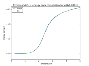
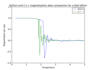
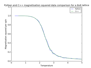
As seen in figure 9, most of the Python data is in agreement with the provided C++ data. The most noticeable difference occurs in the case of magnetisation, since the temperature spacing of the Pyhton data is too large to illustrate the fluctuations occurring at the phase change.

Task 18

Write a script to read the data from a particular file, and plot C vs T, as well as a fitted polynomial. Try changing the degree of the polynomial to improve the fit — in general, it might be difficult to get a good fit! Attach a PNG of an example fit to your report.

from matplotlib import pylab as pl
import numpy as np

lattice_size=input('Lattice size: ')

if lattice_size=='2':
    data=np.loadtxt('C++_data/2x2.dat')
elif lattice_size=='4':
    data=np.loadtxt('C++_data/4x4.dat')
elif lattice_size=='8':
    data=np.loadtxt('C++_data/8x8.dat')
elif lattice_size=='16':
    data=np.loadtxt('C++_data/16x16.dat')
elif lattice_size=='32':
    data=np.loadtxt('C++_data/32x32.dat')
   
T=data[:,0]
C=data[:,5]

#first we fit the polynomial to the data
fit = np.polyfit(T, C, 15) # fit a 15th order polynomial

#now we generate interpolated values of the fitted polynomial over the range of our function
T_min = np.min(T)
T_max = np.max(T)
T_range = np.linspace(T_min, T_max, 1000) #generate 1000 evenly spaced points between T_min and T_max
fitted_C_values = np.polyval(fit, T_range) # use the fit object to generate the corresponding values of C

pl.ylabel("Heat capacity per spin")
pl.xlabel("Temperature")
pl.plot(T,C,label="Data from file")
pl.plot(T_range,fitted_C_values,label="Fitted data")
if lattice_size=='2':
    pl.title('Heat capacity from file versus fitted data for 2x2 lattice')
elif lattice_size=='4':
    pl.title('Heat capacity from file versus fitted data for 4x4 lattice')
elif lattice_size=='8':
    pl.title('Heat capacity from file versus fitted data for 8x8 lattice')
elif lattice_size=='16':
    pl.title('Heat capacity from file versus fitted data for 16x16 lattice')
elif lattice_size=='32':
    pl.title('Heat capacity from file versus fitted data for 32x32 lattice')
pl.legend(loc="best",fontsize="10")
pl.show()

JC: Good use of polyfit and polyval functions.

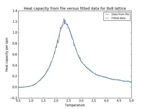
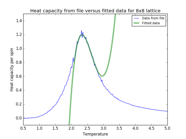
The data was fitted to a 15^th order polynomial for the 2x2 and 4x4 lattice, 20^th order for the 8x8 lattice (figure 10) and 50^th order for the 16x16 and 32x32 lattices.

Task 19

Modify your script from the previous section. You should still plot the whole temperature range, but fit the polynomial only to the peak of the heat capacity! You should find it easier to get a good fit when restricted to this region.

from matplotlib import pylab as pl
import numpy as np

lattice_size=input('Lattice size: ')

if lattice_size=='2':
    data=np.loadtxt('C++_data/2x2.dat')
elif lattice_size=='4':
    data=np.loadtxt('C++_data/4x4.dat')
elif lattice_size=='8':
    data=np.loadtxt('C++_data/8x8.dat')
elif lattice_size=='16':
    data=np.loadtxt('C++_data/16x16.dat')
elif lattice_size=='32':
    data=np.loadtxt('C++_data/32x32.dat')
   
T=data[:,0]
C=data[:,5]

if lattice_size=='2':
    Tmin = 1.7
    Tmax = 3.2
elif lattice_size=='4':
    Tmin = 1.7
    Tmax = 3.2
elif lattice_size=='8':
    Tmin = 2.1
    Tmax = 2.8
elif lattice_size=='16':
    Tmin = 2.0
    Tmax = 2.7
elif lattice_size=='32':
    Tmin = 2.1
    Tmax = 2.6



selection = np.logical_and(T > Tmin, T < Tmax) #choose only those rows where both conditions are true
peak_T_values = T[selection]
peak_C_values = C[selection]

#first we fit the polynomial to the data
fit = np.polyfit(peak_T_values, peak_C_values, 5) #fit to a 5th order polynomial

#now we generate interpolated values of the fitted polynomial over the range of our function
T_min = np.min(T)
T_max = np.max(T)
T_range = np.linspace(T_min, T_max, 1000) #generate 1000 evenly spaced points between T_min and T_max
fitted_C_values = np.polyval(fit, T_range) #use the fit object to generate the corresponding values of C

peak_T_range=np.linspace(Tmin,Tmax,1000) #generate 1000 evenly spaced points between Tmin and Tmax
peak_fitted_C_values=np.polyval(fit,peak_T_range) #use the fit object to generate the corresponding values of C

pl.ylabel("Heat capacity per spin")
pl.xlabel("Temperature")
pl.plot(T,C,label="Data from file")
pl.plot(T_range,fitted_C_values,linewidth=4,alpha=0.5,label="Fitted data")
if lattice_size=='2':
    pl.title('Heat capacity from file versus fitted data for 2x2 lattice')
    pl.ylim(-0.1,0.5)
elif lattice_size=='4':
    pl.title('Heat capacity from file versus fitted data for 4x4 lattice')
    pl.ylim(-0.1,1)

elif lattice_size=='8':
    pl.title('Heat capacity from file versus fitted data for 8x8 lattice')
    pl.ylim(-0.1,1.5)

elif lattice_size=='16':
    pl.title('Heat capacity from file versus fitted data for 16x16 lattice')
    pl.ylim(-0.1,2)

elif lattice_size=='32':
    pl.title('Heat capacity from file versus fitted data for 32x32 lattice')
    pl.ylim(-0.1,2)
   
Cmax = np.max(peak_fitted_C_values) #pick the maximum of the fitted values in the range of the peak
Tmax = peak_T_range[peak_fitted_C_values == Cmax]

print(Tmax)

pl.legend(loc="best",fontsize="10")
pl.show()

The data was fitted to a 5^th order polynomial for the 2x2, 4x4 and 8x8 lattices (figure 11), to a 7^th order polynomial for the 16x16 lattice and to a 10^th order polynomial for the 32x32 lattice.

Task 20

Find the temperature at which the maximum in C occurs for each datafile that you were given. Make a text file containing two colums: the lattice side length (2,4,8, etc.), and the temperature at which C is a maximum. This is your estimate of $T_{C}$ for that side length. Make a plot that uses the scaling relation given above to determine $T_{C, \infty}$ . By doing a little research online, you should be able to find the theoretical exact Curie temperature for the infinite 2D Ising lattice. How does your value compare to this? Are you surprised by how good/bad the agreement is? Attach a PNG of this final graph to your report, and discuss briefly what you think the major sources of error are in your estimate.

**Table 3.** Lattice size and temperature for which the heat capacity is maximum
L	Temperature
2	2.53333333
4	2.44924925
8	2.33333333
16	2.31321321
32	2.29469469

The data in table 3 was saved in LatticeSize_Tmax.dat and used to plot and linearly fit the temperature values as a function of 1/L:

from matplotlib import pylab as pl
import numpy as np

data=np.loadtxt('LatticeSize_Tmax.dat')
L=data[:,0]
Tc=data[:,1]

fit = np.polyfit(1/L, Tc, 1,cov=True)

params=fit[0]
params_cov=fit[1] #the variance for the extracted coefficients

x_range = np.linspace(0, 0.5, 1000) 
fitted_Tc = params[0]*x_range+params[1]

pl.plot(1/L,Tc,linestyle='',marker='o',label="Obtained data")
pl.plot(x_range,fitted_Tc,label="Linear fit")
pl.xlabel("1/L")
pl.ylabel("Curie temperature")
pl.title("Curie temperature versus 1/L for LxL lattices along with linear fit")
pl.legend(loc="best",fontsize="10")
pl.show()

print('T_c_inf = ',fitted_Tc[x_range==0][0],'\nT_c_inf uncertainty = ',params_cov[1,1]**0.5)

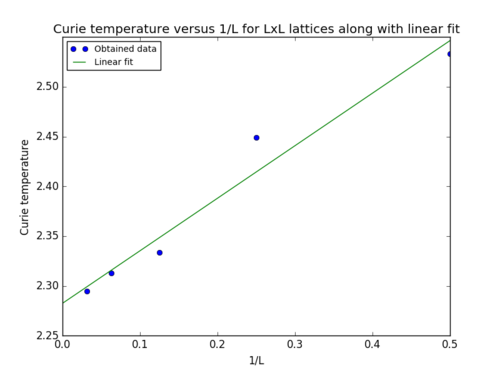
**Figure 12.** Plot of Curie temperature values versus 1/lattice size

The value of the Curie temperature for the infinite 2D lattice determined from the intercept of the linear fit in figure 12 was $T_{C, \infty} = 2.282 \pm 0.027$ . The literature value (2.269) ^[2] lies within the range of the determined value and its uncertainty.

Unsurprisingly, the determined value is therefore in agreement with the analytical solution. Nevertheless, the lack of precision and accuracy can be attributed to the approximations made by employing the Monte Carlo method, which implies that not all possible states are taken into account when determining the average energy. Additionally, the choice for the number of cycles to be ignored from the averaging influences the level of precision of the results. The noise observed in the heat capacity data, especially in the peak region (although fitted to a polynomial) is another source of error which propagated throughout the calculations up to determining the Curie temperature for the infinite 2D lattice as proven by the spread of the data points in figure 12.

JC: Graph looks good, but could you have got a better fit and a closer agreement with the analytical result if you ignored the 2x2 data. You have already shown that this is too small to properly capture the behaviour of the Ising model so could be ignored here.

References

↑ ^1.0 ^1.1 N. W. Ashcroft and N. D. Mermin, Solid State Physics, Harcourt College Publishers, Orlando, 1976.
↑ L. Onsager, Phys. Rev., 1944, 65, 117-149.

[SolidState-1] 1.0 ^1.1 N. W. Ashcroft and N. D. Mermin, Solid State Physics, Harcourt College Publishers, Orlando, 1976.

[Onsager-2] L. Onsager, Phys. Rev., 1944, 65, 117-149.

[1]

[2]