Talk:Mod:ia2514 LiqSim

JC: General comments: All tasks answered well. Try to make your written explanations more specific and focus on the details which are most relevant to explaining the trends that you see in your results.

Third year simulation experiment

This experiment involved performing molecular dynamics simulations for Lennard-Jones systems at various densities, pressures and temperatures, in the microcanonical, canonical and the isobaric-isothermal ensemble in order to investigate the variation of density with temperature at different pressures, to compute the heat capacity and the diffusion coefficient and plot the radial distribution function. The obtained results were correlated with theory and were used to investigate the structure and properties of the systems. All the simulations were run using LAMMPS and the resulting data was further plotted and analysed using Python and Excel. The trends observed in the results were as expected and the values obtained for the diffusion coefficient were in accordance with literature values. A lack of accuracy in some of the results was attributed to the system not reaching equilibrium within the simulated time.

Introduction to molecular dynamics simulation

In this section, the values obtained by employing the Velocity Verlet algorithm for the position of a harmonic oscillator were compared with the classical results and were further used for calculating the total energy of the system. The change in total energy was calculated from the Velocity Verlet solution in order to determine the largest timestep value for which it does not exceed 1%. Various calculations regarding the Lennard-Jones potential, periodic boundary conditions and reduced units were performed.

Task 1

Open the file HO.xls. In it, the velocity-Verlet algorithm is used to model the behaviour of a classical harmonic oscillator. Complete the three columns "ANALYTICAL", "ERROR", and "ENERGY": "ANALYTICAL" should contain the value of the classical solution for the position at time $t$, "ERROR" should contain the absolute difference between "ANALYTICAL" and the velocity-Verlet solution (i.e. ERROR should always be positive -- make sure you leave the half step rows blank!), and "ENERGY" should contain the total energy of the oscillator for the velocity-Verlet solution. Remember that the position of a classical harmonic oscillator is given by $x\left(t\right)=A\cos (\omega t+\varphi )$ (the values of $A$, $\omega$, and $\varphi$ are worked out for you in the sheet).

The energy of the system was calculated as a sum of the potential energy, $\frac{1}{2}k{x}^2$, and the kinetic energy, $\frac{1}{2}m{v}^2$. The filled in file can be found here.

Task 2

For the default timestep value, 0.1, estimate the positions of the maxima in the ERROR column as a function of time. Make a plot showing these values as a function of time, and fit an appropriate function to the data.

Figure 1. Maximum error in the position of the harmonic oscillator as calculated using the Velocity Verlet algorithm and the classical result

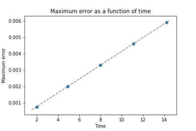
The values of the maxima in the graph of the error (the absolute difference between the analytical solution for the position of the harmonic oscillator with respect to the values obtained from the velocity-Verlet algorithm) as a function of time, along with their corresponding times are presented in table 1 and plotted in figure 1. They occur at time intervals of approximately 3 and can be fitted to a linear function ($4.22\times 10^{-4}\times t-7.78\times 10^{-5}$).

JC: Why do you think the error oscillates over time even though the height of the maximum error increases?

Table 1. Error maxima: classical result versus the Velocity Verlet solution

Time	Error
2.00	7.58E-4
4.90	2.01E-3
8.00	3.30E-3
11.10	4.60E-3
14.20	5.91E-3

Task 3

Experiment with different values of the timestep. What sort of a timestep do you need to use to ensure that the total energy does not change by more than 1% over the course of your "simulation"? Why do you think it is important to monitor the total energy of a physical system when modelling its behaviour numerically?

Monitoring the total energy of the system is important for ensuring that the system has reached equilibrium. The variation in the total energy increases with the value of the timestep and a timestep of 0.334 leads to a change in the total energy of 1.00%. Therefore, in order to ensure that the energy does not change by more than 1% the timestep should be set to less than 0.334.

JC: Energy must be conserved, approximately, for the simulation to give physically relevant results.

Task 4

For a single Lennard-Jones interaction, $\varphi \left(r\right)=4ϵ(\frac{{\sigma }^{12}}{r^{12}}-\frac{{\sigma }^6}{r^6})$, find the separation, $r_0$, at which the potential energy is zero. What is the force at this separation? Find the equilibrium separation, $r_{eq}$, and work out the well depth ($\varphi \left(r_{eq}\right)$). Evaluate the integrals $\underset{2\sigma }{\overset{\mathrm{\infty }}{\int }}\varphi \left(r\right)\mathrm{d}r$, $\underset{2.5\sigma }{\overset{\mathrm{\infty }}{\int }}\varphi \left(r\right)\mathrm{d}r$, and $\underset{3\sigma }{\overset{\mathrm{\infty }}{\int }}\varphi \left(r\right)\mathrm{d}r$ when $\sigma =ϵ=1.0$.

$\bullet$ The separation, $r_0$, at which the potential energy is zero is:

$\varphi \left(r_0\right)=0\Rightarrow 4ϵ(\frac{{\sigma }^{12}}{r_0^{12}}-\frac{{\sigma }^6}{r_0^6})=0\iff \frac{{\sigma }^{12}}{r_0^{12}}=\frac{{\sigma }^6}{r_0^6}\Rightarrow r_0^6={\sigma }^6\Rightarrow r_0=\sigma$ (since $r_0>0$ and $\sigma >0$)

$\bullet$ The force at this separation is:

$F(r)=-\frac{\mathrm{d}\varphi \left(r\right)}{\mathrm{d}r}\Rightarrow F(r)=-\frac{\mathrm{d}\left[4ϵ(\frac{{\sigma }^{12}}{r^{12}}-\frac{{\sigma }^6}{r^6})\right]}{\mathrm{d}r}\iff F(r)=\frac{24ϵ}{\sigma }[2{\left(\frac{\sigma }{r}\right)}^{13}-{\left(\frac{\sigma }{r}\right)}^7]$

$\Rightarrow F(r_0)=\frac{24ϵ}{\sigma }$

$\bullet$ At equilibrium, $F(r_{eq})=0\Rightarrow \frac{24ϵ}{\sigma }[2{\left(\frac{\sigma }{r_{eq}}\right)}^{13}-{\left(\frac{\sigma }{r_{eq}}\right)}^7]=0\Rightarrow 2{\left(\frac{\sigma }{r_{eq}}\right)}^{13}-{\left(\frac{\sigma }{r_{eq}}\right)}^7=0\Rightarrow 2{\sigma }^6=r_{eq}^6\Rightarrow r_{eq}=\sqrt[6]{2}\sigma$

$\bullet$ $r_{eq}=\sqrt[6]{2}\sigma \Rightarrow \varphi \left(r_{eq}\right)=4ϵ(\frac{{\sigma }^{12}}{4{\sigma }^{12}}-\frac{{\sigma }^6}{2{\sigma }^6})\Rightarrow \varphi \left(r_{eq}\right)=-ϵ$

$\begin{array}{rl}\bullet \underset{2\sigma }{\overset{\mathrm{\infty }}{\int }}\varphi \left(r\right)\mathrm{d}r& =\underset{2\sigma }{\overset{\mathrm{\infty }}{\int }}4ϵ(\frac{{\sigma }^{12}}{r^{12}}-\frac{{\sigma }^6}{r^6})\mathrm{d}r\\ & =4ϵ{\sigma }^{12}\underset{2\sigma }{\overset{\mathrm{\infty }}{\int }}{r}^{-12}\mathrm{d}r-4ϵ{\sigma }^6\underset{2\sigma }{\overset{\mathrm{\infty }}{\int }}{r}^{-6}\mathrm{d}r\\ & ={-\frac{4ϵ{\sigma }^{12}}{11}{r}^{-11}|}_{2\sigma }^{\mathrm{\infty }}+{\frac{4ϵ{\sigma }^6}{5}{r}^{-5}|}_{2\sigma }^{\mathrm{\infty }}\\ & =\frac{4ϵ{\sigma }^{12}}{11}{\left(2\sigma \right)}^{-11}-\frac{4ϵ{\sigma }^6}{5}{\left(2\sigma \right)}^{-5}\\ & =\frac{4ϵ\sigma }{11\times 2^{11}}-\frac{4ϵ\sigma }{5\times 2^5}\\ & =\frac{(5-11\times 2^6)ϵ\sigma }{5\times 11\times 2^9}\end{array}$

For σ = ϵ = 1.0, $\underset{2\sigma }{\overset{\mathrm{\infty }}{\int }}\varphi \left(r\right)\mathrm{d}r=-0.02482$

$\begin{array}{rl}\bullet \underset{2.5\sigma }{\overset{\mathrm{\infty }}{\int }}\varphi \left(r\right)\mathrm{d}r& =\underset{2.5\sigma }{\overset{\mathrm{\infty }}{\int }}4ϵ(\frac{{\sigma }^{12}}{r^{12}}-\frac{{\sigma }^6}{r^6})\mathrm{d}r\\ & =4ϵ{\sigma }^{12}\underset{2.5\sigma }{\overset{\mathrm{\infty }}{\int }}{r}^{-12}\mathrm{d}r-4ϵ{\sigma }^6\underset{2.5\sigma }{\overset{\mathrm{\infty }}{\int }}{r}^{-6}\mathrm{d}r\\ & ={-\frac{4ϵ{\sigma }^{12}}{11}{r}^{-11}|}_{2.5\sigma }^{\mathrm{\infty }}+{\frac{4ϵ{\sigma }^6}{5}{r}^{-5}|}_{2.5\sigma }^{\mathrm{\infty }}\\ & =\frac{4ϵ{\sigma }^{12}}{11}{(2.5\sigma )}^{-11}-\frac{4ϵ{\sigma }^6}{5}{(2.5\sigma )}^{-5}\\ & =\frac{4ϵ\sigma }{11\times 2.5^{11}}-\frac{4ϵ\sigma }{5\times 2.5^5}\\ \end{array}$

For σ = ϵ = 1.0, $\underset{2.5\sigma }{\overset{\mathrm{\infty }}{\int }}\varphi \left(r\right)\mathrm{d}r=-0.00817$

$\begin{array}{rl}\bullet \underset{3\sigma }{\overset{\mathrm{\infty }}{\int }}\varphi \left(r\right)\mathrm{d}r& =\underset{3\sigma }{\overset{\mathrm{\infty }}{\int }}4ϵ(\frac{{\sigma }^{12}}{r^{12}}-\frac{{\sigma }^6}{r^6})\mathrm{d}r\\ & =4ϵ{\sigma }^{12}\underset{3\sigma }{\overset{\mathrm{\infty }}{\int }}{r}^{-12}\mathrm{d}r-4ϵ{\sigma }^6\underset{3\sigma }{\overset{\mathrm{\infty }}{\int }}{r}^{-6}\mathrm{d}r\\ & ={-\frac{4ϵ{\sigma }^{12}}{11}{r}^{-11}|}_{3\sigma }^{\mathrm{\infty }}+{\frac{4ϵ{\sigma }^6}{5}{r}^{-5}|}_{3\sigma }^{\mathrm{\infty }}\\ & =\frac{4ϵ{\sigma }^{12}}{11}{\left(3\sigma \right)}^{-11}-\frac{4ϵ{\sigma }^6}{5}{\left(3\sigma \right)}^{-5}\\ & =\frac{4ϵ\sigma }{11\times 3^{11}}-\frac{4ϵ\sigma }{5\times 3^5}\\ \end{array}$

For σ = ϵ = 1.0, $\underset{3\sigma }{\overset{\mathrm{\infty }}{\int }}\varphi \left(r\right)\mathrm{d}r=-0.00329$

JC: All maths correct and well laid out.

Task 5

Estimate the number of water molecules in 1ml of water under standard conditions. Estimate the volume of $10000$ water molecules under standard conditions.

Since the density of water under standard conditions is 1 g/mL, the mass of 1 mL of water is m = 1 g.

The number of molecules in 1 mL of water is

$\begin{array}{rl}N& =\frac{m\times N_{\mathrm{A}}}{\mu }\\ & =\frac{1\times 6.022\times 10^{23}}{18.015}\\ & =3.34\times 10^{22}\\ \end{array}$

The mass of N=10000 water molecules is

$\begin{array}{rl}m& =\frac{N\times \mu }{N_{\mathrm{A}}}\\ & =\frac{10000\times 18.015}{6.022\times 10^{23}}\\ & =2.99\times 10^{-19}\mathrm{g}\\ \end{array}$

The volume of 10000 water molecules under standard conditions is therefore $V=1\frac{\mathrm{g}}{\mathrm{m}\mathrm{L}}\times 2.99\times 10^{-19}\mathrm{g}=2.99\times 10^{-19}\mathrm{m}\mathrm{L}$.

Task 6

Consider an atom at position $(0.5,0.5,0.5)$ in a cubic simulation box which runs from $(0,0,0)$ to $(1,1,1)$. In a single timestep, it moves along the vector $(0.7,0.6,0.2)$. At what point does it end up, after the periodic boundary conditions have been applied?

After moving along the vector $(0.7,0.6,0.2)$, the atom ends up at $(0.5,0.5,0.5)+(0.7,0.6,0.2)=(1.2,1.1,0.7)$. By applying the periodic boundary conditions, this is equivalent to $(1.2mod1,1.1mod1,0.7mod1)=(0.2,0.1,0.7)$.

Task 7

The Lennard-Jones parameters for argon are $$\begin{gathered} \sigma =0.34\mathrm{n}\mathrm{m},ϵ \\ / \\ {k}_B=120\mathrm{K} \end{gathered}$$. If the LJ cutoff is $r^{*}=3.2$, what is it in real units? What is the well depth in $$\begin{gathered} {\mathrm{k}\mathrm{J} \\ \mathrm{m}\mathrm{o}\mathrm{l}}^{-1} \end{gathered}$$? What is the reduced temperature $T^{*}=1.5$ in real units?

$r^{*}=\frac{r}{\sigma }\Rightarrow r=r^{*}\times \sigma \Rightarrow r=3.2\times 0.34\mathrm{n}\mathrm{m}=1.088\mathrm{n}\mathrm{m}$

The well depth is $ϵ=k_{\mathrm{B}}\times \frac{ϵ}{k_{\mathrm{B}}}\Rightarrow ϵ=1.38\times 10^{-23}\times 120=1.656\times 10^{-21}\mathrm{J}\Rightarrow ϵ=1.656\times 10^{-21}\times 10^{-3}\times N_{\mathrm{A}}=1.00\mathrm{k}\mathrm{J}/\mathrm{m}\mathrm{o}\mathrm{l}$.

The temperature is $T=T^{*}\times \frac{ϵ}{k_{\mathrm{B}}}\Rightarrow T=1.5\times 120=180\mathrm{K}$.

JC: All calculations correct and working clearly shown.

Equilibration

Simulations for the same system (in the microcanonical ensemble) at five different timesteps (0.001, 0.0025, 0.0075, 0.01, 0.015) were performed and various commands within the input files were explained. The energy, pressure and temperature were plotted against time for the five timestep values which allowed for the selection of an optimum timestep to be used in further simulations.

Task 8

Why do you think giving atoms random starting coordinates causes problems in simulations? Hint: what happens if two atoms happen to be generated close together?

Setting up a simulation with random coordinates could generate atoms that are too close together (at a distance lower than the sum of their Van der Waals radii), which would lead to strong repulsion. The probability of creating overlapping atoms is higher for more dense systems.

JC: What would be the problem with strong repulsive forces? Large forces can make the simulation unstable and cause it to crash unless much smaller timesteps are used.

Task 9

Satisfy yourself that this lattice spacing corresponds to a number density of lattice points of $0.8$. Consider instead a face-centred cubic lattice with a lattice point number density of 1.2. What is the side length of the cubic unit cell?

Since the density $\frac{N}{V}=0.8$ and $N=1$ (because it is a simple cubic lattice), the volume of the unit lattice is $V=\frac{1}{0.8}=1.25$ and therefore $L^3=1.25\Rightarrow L=1.07722$.

In the case of a FCC lattice (for which $N=4$) with a lattice point number density of 1.2, the volume is $V=\frac{4}{1.2}=3.33$ which gives a side length of the cubic unit cell of $L=\sqrt[3]{3.33}=1.49380$.

Task 10

Consider again the face-centred cubic lattice from the previous task. How many atoms would be created by the create_atoms command if you had defined that lattice instead?

For a face-centred cubic lattice the number of lattice points per unit cell is 4, and therefore for a 10x10x10 box, the create_atoms command would create 4x10x10x10=4000 atoms.

JC: Correct.

Task 11

Using the LAMMPS manual, find the purpose of the following commands in the input script:

mass 1 1.0
pair_style lj/cut 3.0
pair_coeff * * 1.0 1.0

The mass 1 1.0 command sets the mass of all the atoms of type 1 to 1.0 (in this case, all the atoms are of type 1, as set in the command create_atoms 1 box).

The pair_style lj/cut 3.0 command models the interactions between each pair of atoms using the standard Lennard-Jones potential, $\varphi \left(r\right)=4ϵ(\frac{{\sigma }^{12}}{r^{12}}-\frac{{\sigma }^6}{r^6})$ with a cutoff of 3.0 (i.e. the potential is calculated only for $r<3.0$; above this value it is 0).

The pair_coeff * * 1.0 1.0 command sets $ϵ=1.0$ and $\sigma =1.0$ for all the possible pairs of atoms (the asterisk represents all the atom types).

All the aforementioned values are in reduced units.

JC: Well explained, why is a cutoff used for this potential?

Task 12

Given that we are specifying ${\mathbf{x}}_i\left(0\right)$ and ${\mathbf{v}}_i\left(0\right)$, which integration algorithm are we going to use?

Since both the position ${\mathbf{x}}_i\left(0\right)$ and velocity ${\mathbf{v}}_i\left(0\right)$ are used as initial conditions, the Velocity Verlet Algorithm will be used.

Task 13

Look at the lines below.

### SPECIFY TIMESTEP ###
variable timestep equal 0.001
variable n_steps equal floor(100/${timestep})
variable n_steps equal floor(100/0.001)
timestep ${timestep}
timestep 0.001

### RUN SIMULATION ###
run ${n_steps}
run 100000

The second line (starting "variable timestep...") tells LAMMPS that if it encounters the text ${timestep} on a subsequent line, it should replace it by the value given. In this case, the value ${timestep} is always replaced by 0.001. In light of this, what do you think the purpose of these lines is? Why not just write:

timestep 0.001
run 100000

The purpose of using ${timestep} instead of 0.001 (i.e. using a variable instead of a numeric value) is to facilitate using the same script with different values and ensure consistency. By using variables, any change in values has to be done only once (when assigning the values to the variable) and any mistakes in replacing the numbers manually are avoided.

JC: Correct.

Task 14

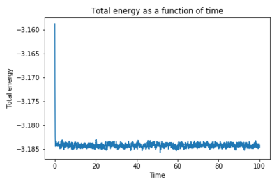
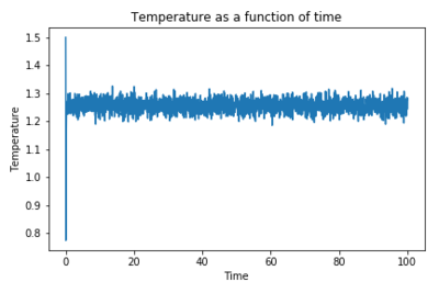
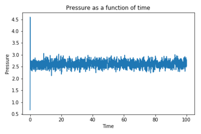
Make plots of the energy, temperature, and pressure, against time for the 0.001 timestep experiment (attach a picture to your report). Does the simulation reach equilibrium? How long does this take? When you have done this, make a single plot which shows the energy versus time for all of the timesteps (again, attach a picture to your report). Choosing a timestep is a balancing act: the shorter the timestep, the more accurately the results of your simulation will reflect the physical reality; short timesteps, however, mean that the same number of simulation steps cover a shorter amount of actual time, and this is very unhelpful if the process you want to study requires observation over a long time. Of the five timesteps that you used, which is the largest to give acceptable results? Which one of the five is a particularly bad choice? Why?

Figure 2. Total energy versus time for a timestep of 0.001	Figure 3. Temperature versus time for a timestep of 0.001	Figure 4. Pressure versus time for a timestep of 0.001
Figure 5. Total energy versus time for a timestep of 0.001 (time 0-2)	Figure 6. Temperature versus time for a timestep of 0.001 (time 0-2)	Figure 7. Pressure versus time for a timestep of 0.001 (time 0-2)

Figure 8. Total energy versus time for various timesteps

As shown in figures 2-4, the system reaches equilibrium since, after an equilibration time, the total energy, temperature and pressure all start fluctuating around a constant equilibrium value. Figures 5-7 illustrate the same graphs for the time interval [0,2], revealing that the system equilibrates after $t\approx 0.5$.

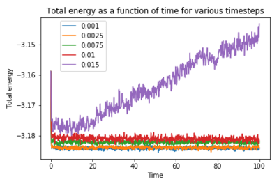
Figure 8 shows a graph of the total energy as a function of time for five different timesteps: 0.001, 0.0025, 0.0075, 0.01 and 0.015. As expected, a smaller timestep minimises the total energy, since it approaches the behaviour of a real physical system, so the lowest total energy is obtained for a timestep of 0.001. A timestep of 0.0025 gives an average total energy at equilibrium that is within 0.0045% of the value obtained in the case of a timestep of 0.001, deeming it a suitable choice for further simulations as it allows for a shorter computational time (less timesteps) than a timestep of 0.001 (for the same simulation time) while yielding reasonably accurate results.

Another notable feature of the plot in figure 8 is the fact that an increase in the size of the timestep eventually leads to non-equilibration: in the case of a timestep of 0.015, the system does not reach equilibrium within the time $\mathrm{\Delta }t=100$, its average total energy increasing steadily after the initial decrease. A timestep of 0.015 is therefore not a good choice for simulating such a system.

JC: Good, the average total energy should not depend on the timestep, so 0.0025 is the best choice.

Running simulations under specific conditions

In this section, performing simulations at seven temperatures and three pressures in the NpT ensemble allowed for the investigation of the variation of density with temperature and a comparison with results obtained from the ideal gas equation.

Task 15

Choose 5 temperatures (above the critical temperature $T^{*}=1.5$), and two pressures (you can get a good idea of what a reasonable pressure is in Lennard-Jones units by looking at the average pressure of your simulations from the last section). This gives ten phase points — five temperatures at each pressure. Create 10 copies of npt.in, and modify each to run a simulation at one of your chosen $(p,T)$ points. You should be able to use the results of the previous section to choose a timestep. Submit these ten jobs to the HPC portal. While you wait for them to finish, you should read the next section.

Simulations were run for seven different temperatures: 1.6, 1.7, 1.8, 1.9, 2.0, 2.2 and 2.4 at three different pressures: 2.5, 3.0 and 3.5 and with a timestep of 0.0025, which was previously selected to be a suitable value.

Task 16

We need to choose $\gamma$ so that the temperature is correct $T=\mathfrak{𝔗}$ if we multiply every velocity $\gamma$. We can write two equations:

$\frac{1}{2}\sum _i{m}_i{v}_i^2=\frac{3}{2}N{k}_{B}T$

$\frac{1}{2}\sum _i{m}_i{\left(\gamma v_i\right)}^2=\frac{3}{2}N{k}_B\mathfrak{𝔗}$

Solve these to determine $\gamma$.

Since $\gamma$ is a constant, it can be taken out of the sum: $\frac{1}{2}\sum _i{m}_i{\left(\gamma v_i\right)}^2=\frac{3}{2}N{k}_B\mathfrak{𝔗}\Rightarrow {\gamma }^2\frac{1}{2}\sum _i{m}_i{v}_i^2=\frac{3}{2}N{k}_B\mathfrak{𝔗}$.

Replacing the sum from the first equation gives ${\gamma }^2\frac{3}{2}N{k}_{B}T=\frac{3}{2}N{k}_B\mathfrak{𝔗}\Rightarrow \gamma =\pm \sqrt{\frac{\mathfrak{𝔗}}{T}}$.

Given that $\gamma >0$, it follows that $\gamma =\sqrt{\frac{\mathfrak{𝔗}}{T}}$.

JC: Good.

Task 17

Use the manual page to find out the importance of the three numbers 100 1000 100000. How often will values of the temperature, etc., be sampled for the average? How many measurements contribute to the average? Looking to the following line, how much time will you simulate?

The three number arguments of fix ave/time represent (in order) the number of steps elapsed between sampling values for the average, the number of values that contribute to the average and the number of steps after which the average is computed. The values of temperature, etc. are therefore sampled every 100 steps for the average and 1000 out of these measurements contribute to the average, which is calculated every 100000 steps.

The simulation will run for 100000 steps (run 100000) and hence, for a timestep of 0.0025, the time that will be simulated is $100000\times 0.0025=250$.

Figure 9. Density as a function of temperature at three different pressures (both simulation results and ideal gas)

Task 18

When your simulations have finished, download the log files as before. At the end of the log file, LAMMPS will output the values and errors for the pressure, temperature, and density $\left(\frac{N}{V}\right)$. Use software of your choice to plot the density as a function of temperature for both of the pressures that you simulated. Your graph(s) should include error bars in both the x and y directions. You should also include a line corresponding to the density predicted by the ideal gas law at that pressure. Is your simulated density lower or higher? Justify this. Does the discrepancy increase or decrease with pressure?

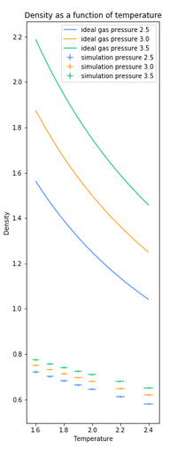
Figure 9 shows the expected trend in the values of the density as a function of temperature: for all three pressures simulated, the density decreases with an increase in temperature. The plot also displays the density as obtained from the ideal gas equation ($\frac{N^{*}}{V^{*}}=\frac{p^{*}}{T^{*}}$) and as expected, the values obtained from the Lennard-Jones systems are lower than those calculated for an ideal gas, for all three pressures. This discrepancy can be explained through the approximations made when considering an ideal gas: the interactions between the particles are purely elastic, whereas the Lennard-Jones potential takes into account the attractive forces between the particles (as well as the repulsive ones). The difference between the ideal gas and the Lennard-Jones densities also increase with an increase in pressure and decrease in temperature (which is consistent with the fact that the ideal gas theory works best for very dilute gases, reduced pressures and high temperatures): for a pressure of 2.5 the difference decreases with temperature from 0.84 to 0.46, whereas for a pressure of 3.5, this difference ranges from 1.41 to 0.81.

JC: The main approximation in the ideal gas equation that is relevant here is the lack of repulsive forces which means that particles in an ideal gas can be at much higher densities than in a Lennard-Jones gas, attractive forces are not very significant in a gas. Try to be a bit more specific in your answer.

Calculating heat capacities using statistical physics

The change in heat capacity per volume with temperature was studied using the results obtained from running simulations for a Lennard-Jones system at five different temperatures and two density values.

Task 19

As in the last section, you need to run simulations at ten phase points. In this section, we will be in density-temperature $({\rho }^{*},T^{*})$ phase space, rather than pressure-temperature phase space. The two densities required at $0.2$ and $0.8$, and the temperature range is $2.0,2.2,2.4,2.6,2.8$. Plot $C_V/V$ as a function of temperature, where $V$ is the volume of the simulation cell, for both of your densities (on the same graph). Is the trend the one you would expect? Attach an example of one of your input scripts to your report.

Figure 10. Heat capacity per volume versus temperature for two different densities

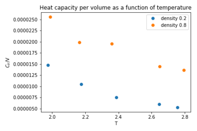
The trend shown in figure 10 is the one expected: the heat capacity decreases with temperature for both densities. This observation can be explained through the fact that at higher temperatures, the particles vibrate more, the interactions between them become weaker and therefore they can store less energy, leading to a decrease in their heat capacity. Between the two data sets, it can be observed that heat capacity increases with increasing density, since a higher density implies a larger number of particles per unit volume which can therefore store more energy, which is consistent with the fact that heat capacity is an extensive property.

JC: Good explanation of the trend with density. For the trend with temperature, if particles vibrate more won't they store more kinetic energy? The change in heat capacity with temperature can be related to the density of states, but more analysis is needed to recover this.

### SPECIFY THE REQUIRED THERMODYNAMIC STATE ###
variable T equal 2.0
variable timestep equal 0.0025
variable dens equal 0.2

### DEFINE SIMULATION BOX GEOMETRY ###
lattice sc ${dens}
region box block 0 15 0 15 0 15
create_box 1 box
create_atoms 1 box

### DEFINE PHYSICAL PROPERTIES OF ATOMS ###
mass 1 1.0
pair_style lj/cut/opt 3.0
pair_coeff 1 1 1.0 1.0
neighbor 2.0 bin

### ASSIGN ATOMIC VELOCITIES ###
velocity all create ${T} 12345 dist gaussian rot yes mom yes

### SPECIFY ENSEMBLE ###
timestep ${timestep}
fix nve all nve

### THERMODYNAMIC OUTPUT CONTROL ###
thermo_style custom time etotal temp press
thermo 10

### RECORD TRAJECTORY ###
dump traj all custom 1000 output-1 id x y z

### SPECIFY TIMESTEP ###

### RUN SIMULATION TO MELT CRYSTAL ###
run 10000
unfix nve
reset_timestep 0

### BRING SYSTEM TO REQUIRED STATE ###
variable tdamp equal ${timestep}*100
fix nvt all nvt temp ${T} ${T} ${tdamp} 
run 10000
reset_timestep 0

### SWITCH OFF THERMOSTAT ###
unfix nvt
fix nve all nve

### MEASURE SYSTEM STATE ###
thermo_style custom step etotal temp vol density atoms
variable dens equal density
variable N equal atoms
variable N2 equal atoms*atoms
variable temp equal temp
variable temp2 equal temp*temp
variable vol equal vol
variable en equal etotal
variable en2 equal etotal*etotal
fix aves all ave/time 100 1000 100000 v_dens v_temp v_vol v_en v_en2 v_temp2
run 100000

variable avedens equal f_aves[1]
variable avetemp equal f_aves[2]
variable avevol equal f_aves[3]
variable aveen equal f_aves[4]
variable aveen2 equal f_aves[5]
variable varen equal f_aves[5]-f_aves[4]*f_aves[4]
variable heatcap equal ${N2}*${varen}/f_aves[6]


print "Averages"
print "--------"
print "Density: ${avedens}"
print "Temperature: ${avetemp}"
print "Volume: ${avevol}"
print "Energy: ${aveen}"
print "N2: ${N2}"
print "Var Energy: ${varen}"
print "Heat Capacity: ${heatcap}"

Structural properties and the radial distribution function

Density and temperature values for the vapour, liquid and solid phases of a Lennard-Jones system were extracted from the phase diagram and used to compute the radial distribution function for the three states. Plots of the RDFs allowed for correlations with the structure of the system in each phase.

Task 20

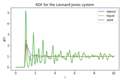
Perform simulations of the Lennard-Jones system in the three phases. When each is complete, download the trajectory and calculate $g(r)$ and $\int g(r)\mathrm{d}r$. Plot the RDFs for the three systems on the same axes, and attach a copy to your report. Discuss qualitatively the differences between the three RDFs, and what this tells you about the structure of the system in each phase. In the solid case, illustrate which lattice sites the first three peaks correspond to. What is the lattice spacing? What is the coordination number for each of the first three peaks?

Table 2. Parameters used for the Lennard-Jones system

Phase	Density	Temperature
vapour	0.07	1.3
liquid	0.80	1.2
solid	1.20	0.8

The densities and temperatures for the solid and vapour systems were extracted from the Lennard-Jones system phase diagram and are presented in table 2.

Figure 11. RDF versus distance for a Lennard-Jones system in vapour, liquid and solid state

Figure 12. RDF integral versus distance for a Lennard-Jones system in vapour, liquid and solid state

Figure 13. FCC lattice showing the corresponding positions of the first three peaks in the RDF graph

The radial distribution functions for vapour, liquid and solid Lennard-Jones systems are shown in figure 11 and present the expected features. At distances lower than the minimum interatomic distance, the RDF is zero for all three cases. The solid system, the most ordered one, presents sharp peaks corresponding to certain positions in the FCC lattice. The intensity of the peaks decreases with an increase in the radius suggesting a decrease in the long-range order, which can be attributed to thermal motion. The liquid system is not as ordered as the solid one (it only displays short-range order), but still presents a few peaks at low distances after which the RDF falls to 1, indicating a similar density in the spherical shell at distance r as in the bulk, and therefore a lack of long-range ordering of the system. The RDF for the vapour case is the one which falls to 1 at the lowest distance out of the three cases, an observation which is consistent with the lack of ordering observed in the gas phase. Given the differences between the RDF plots for the three systems, it is expected that the running integral for the vapour reaches a plateau before the liquid, which in turn reaches a constant value before the solid. These features are confirmed by the graph in figure 12.

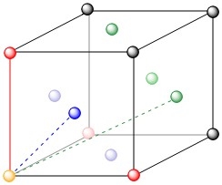
In the case of a solid system, the first RDF peaks represent the nearest neighbour shells. For a FCC lattice, we expect the first three peaks in the RDF to occur at r values corresponding to the distances between the yellow particle (the centre) and the blue, red and green particles in figure 13 as these are the first three closest particles to the centre. The values of the r distances for the first three RDF peaks, which approximately correspond to the predicted values, along with the corresponding distance to the centre as a function of the lattice spacing $L=1.4938$ (extracted from the log file of the simulation for the solid system) and the coordination numbers (calculated by considering the number of atoms per unit cell and the number of neighbouring cells) are presented in table 3.

Table 3. Lattice sites to which the first three peaks correspond to

r value	Distance from centre as a function of L	Coordination number
1.025	$L\frac{\sqrt{2}}{2}$	12
1.475	$L$	6
1.825	$L\sqrt{\frac{3}{2}}$	24

JC: The running integral should not reach a plateau, but should reach a straight line with constant gradient as the RDF tends to 1, not zero. The peaks in the solid RDF decrease over time because the volume of the spherical shell used in the calculation of the RDF increases more quickly than the number of atoms at a given distance. Good diagram of an fcc lattice and good idea to use each of the first 3 peaks to compare with the lattice parameters, but you should show how well they agree - what is the lattice parameter predicted from each of the first 3 peaks?

Dynamical properties and the diffusion coefficient

The mean square displacement and the velocity autocorrelation function were extracted from the outputs of simulations for the vapour, liquid and solid Lennard-Jones systems. The features of the plots of both MSD and VACF against time were discussed in correlation to the structures of the system in the three phases. The VACF of the Lennard-Jones system was also compared to the calculated VACF of a 1D harmonic oscillator. The diffusion coefficient was computed using both the MSD and VACF and the results were similar and consistent with literature values. The lack of accuracy in some of the results obtained by using the VACF were attributed to the systems not reaching equilibrium by the end of the simulation.

Task 21

In the D subfolder, there is a file liq.in that will run a simulation at specified density and temperature to calculate the mean squared displacement and velocity autocorrelation function of your system. Run one of these simulations for a vapour, liquid, and solid. You have also been given some simulated data from much larger systems (approximately one million atoms). You will need these files later.

The parameters used for the vapour, liquid and solid are presented in table 2.

Task 22

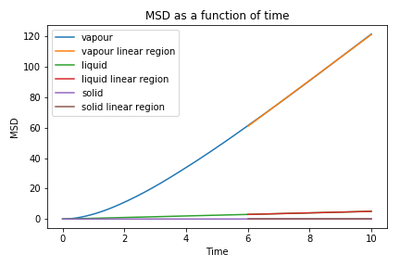
Make a plot for each of your simulations (solid, liquid, and gas), showing the mean squared displacement (the "total" MSD) as a function of timestep. Are these as you would expect? Estimate $D$ in each case. Be careful with the units! Repeat this procedure for the MSD data that you were given from the one million atom simulations.

Figure 14. MSD versus time for a Lennard-Jones system in vapour, liquid and solid state

Figure 15. MSD versus time for a Lennard-Jones system in vapour, liquid and solid state (one million atoms)

The plots in figures 14-15 present the expected features: the mean square displacement increases in the order solid < liquid << vapour, in accordance with the freedom of movement for the particles in each of the three states. After a period of time, they all exhibit a linear behaviour, with the vapour MSD gradient being the highest of the three and the solid MSD having an approximately constant value close to 0. The non-linear region at small t values represents the ballistic regime where, in the time before a particle collides with another particle, its velocity can be considered constant and therefore its MSD varies with t², leading to a parabolic curve at low t.

The data points in the time interval [6,10] were each fitted to a linear function and the resulting gradients were used to calculate the diffusion coefficient according to the equation $D=\frac{1}{6}\frac{\partial ⟨r^2\left(t\right)⟩}{\partial t}$. The results are summarised in table 4 and their magnitudes reflect the ease of diffusion within each phase: the diffusion coefficient for the vapour phase is higher than for the liquid and the one for the solid state is close to 0. The values obtained from the two data sets are similar, with the largest difference being observed in the case of the vapour phase (the smaller system yielded a diffusion coefficient value that is 20% smaller than the one calculated from the million atom simulation). Nevertheless, the values obtained for the diffusion coefficient are in accordance with previously reported values obtained through a similar method.

Table 4. Diffusion coefficient calculated using the MSD

Data set	Diffusion coefficient
	Vapour	Liquid	Solid
8000/32000 atoms	2.51	8.48x10-2	-6.66x10-6
1000000 atoms	3.14	8.90x10-2	1.22x10-6
literature	3.694 (at density 0.05); 1.798 (at density 0.10)	7.9x10-2	-

JC: Very good explanation of the ballistic regime. Show the different phases on different plots as it is difficult to see the shape of the solid or liquid MSD from those plots.

Task 23

In the theoretical section at the beginning, the equation for the evolution of the position of a 1D harmonic oscillator as a function of time was given. Using this, evaluate the normalised velocity autocorrelation function for a 1D harmonic oscillator (it is analytic!):

$C\left(\tau \right)=\frac{\underset{-\mathrm{\infty }}{\overset{\mathrm{\infty }}{\int }}v\left(t\right)v(t+\tau )\mathrm{d}t}{\underset{-\mathrm{\infty }}{\overset{\mathrm{\infty }}{\int }}{v}^2\left(t\right)\mathrm{d}t}$

Be sure to show your working in your writeup. On the same graph, with x range 0 to 500, plot $C\left(\tau \right)$ with $\omega =1/2\pi$ and the VACFs from your liquid and solid simulations. What do the minima in the VACFs for the liquid and solid system represent? Discuss the origin of the differences between the liquid and solid VACFs. The harmonic oscillator VACF is very different to the Lennard Jones solid and liquid. Why is this? Attach a copy of your plot to your writeup.

$x\left(t\right)=A\cos (\omega t+\varphi )$ and $v\left(t\right)=\frac{\mathrm{d}x\left(t\right)}{\mathrm{d}t}\Rightarrow v\left(t\right)=-A\omega sin(\omega t+\varphi )$

$\begin{array}{rl}C\left(\tau \right)& =\frac{\underset{-\mathrm{\infty }}{\overset{\mathrm{\infty }}{\int }}[-A\omega sin(\omega t+\varphi )][-A\omega sin(\omega t+\omega \tau +\varphi )]\mathrm{d}t}{\underset{-\mathrm{\infty }}{\overset{\mathrm{\infty }}{\int }}{[-A\omega sin(\omega t+\varphi )]}^2\mathrm{d}t}\\ & =\frac{\frac{A^2{\omega }^2}{2}\underset{-\mathrm{\infty }}{\overset{\mathrm{\infty }}{\int }}[cos\left(\omega \tau \right)-cos(2\omega t+\omega \tau +2\varphi )]\mathrm{d}t}{\frac{A^2{\omega }^2}{2}\underset{-\mathrm{\infty }}{\overset{\mathrm{\infty }}{\int }}[1-cos(2\omega t+2\varphi )]\mathrm{d}t}\mathrm{(}\mathrm{u}\mathrm{s}\mathrm{i}\mathrm{n}\mathrm{g}sin\left(a\right)sin\left(b\right)=\frac{1}{2}[cos(a-b)-cos(a+b)]\mathrm{)}\\ & =\frac{\underset{-\mathrm{\infty }}{\overset{\mathrm{\infty }}{\int }}[cos\left(\omega t\right)-cos\left(\omega \tau \right)cos(2\omega t+2\varphi )+sin\left(\omega \tau \right)sin(2\omega t+2\varphi )]\mathrm{d}t}{\underset{-\mathrm{\infty }}{\overset{\mathrm{\infty }}{\int }}[1-cos(2\omega t+2\varphi )]\mathrm{d}t}\mathrm{(}\mathrm{u}\mathrm{s}\mathrm{i}\mathrm{n}\mathrm{g}cos(a+b)=cos\left(a\right)cos\left(b\right)-sin\left(a\right)sin\left(b\right)\mathrm{)}\\ & =\frac{cos\left(\omega \tau \right)\underset{-\mathrm{\infty }}{\overset{\mathrm{\infty }}{\int }}[1-cos(2\omega t+2\varphi )]\mathrm{d}t+sin\left(\omega \tau \right)\underset{-\mathrm{\infty }}{\overset{\mathrm{\infty }}{\int }}sin(2\omega t+2\varphi )\mathrm{d}t}{\underset{-\mathrm{\infty }}{\overset{\mathrm{\infty }}{\int }}[1-cos(2\omega t+2\varphi )]\mathrm{d}t}\\ & =cos\left(\omega \tau \right)+sin\left(\omega \tau \right)\frac{\underset{-\mathrm{\infty }}{\overset{\mathrm{\infty }}{\int }}sin(2\omega t+2\varphi )\mathrm{d}t}{\underset{-\mathrm{\infty }}{\overset{\mathrm{\infty }}{\int }}[1-cos(2\omega t+2\varphi )]\mathrm{d}t}\\ & =cos\left(\omega \tau \right)+sin\left(\omega \tau \right)\frac{\frac{-1}{2\omega }{\left[cos(2\omega t+2\varphi )\right]}_{-\mathrm{\infty }}^{\mathrm{\infty }}}{{\left[t\right]}_{-\mathrm{\infty }}^{\mathrm{\infty }}-\frac{1}{2\omega }{\left[sin(2\omega t+2\varphi )\right]}_{-\mathrm{\infty }}^{\mathrm{\infty }}}\end{array}$

${\left[cos(2\omega t+2\varphi )\right]}_{-\mathrm{\infty }}^{\mathrm{\infty }}$ and ${\left[sin(2\omega t+2\varphi )\right]}_{-\mathrm{\infty }}^{\mathrm{\infty }}$ are finite numbers, ${\left[t\right]}_{-\mathrm{\infty }}^{\mathrm{\infty }}\to \mathrm{\infty }$ and therefore, $\frac{\frac{-1}{2\omega }{\left[cos(2\omega t+2\varphi )\right]}_{-\mathrm{\infty }}^{\mathrm{\infty }}}{{\left[t\right]}_{-\mathrm{\infty }}^{\mathrm{\infty }}-\frac{1}{2\omega }{\left[sin(2\omega t+2\varphi )\right]}_{-\mathrm{\infty }}^{\mathrm{\infty }}}\to 0$ which leads to $C\left(\tau \right)=cos\left(\omega \tau \right)$

JC: Correct result, you can simplify the derivation by recognising integrands as even or odd functions and canceling them accordingly.

Figure 16. VACF versus time for a Lennard-Jones system in vapour, liquid and solid state

Figure 17. VACF versus time for a Lennard-Jones system in vapour, liquid and solid state (one million atoms)

The evolution of the velocity autocorrelation function with time is shown in figures 16-17. In the case of the vapour phase, the VACF decays exponentially with time, indicating a decrease in the correlation between the velocity at time t and the initial velocity which is consistent with the fact that the velocity of a particle is continually changed due to the weak intermolecular forces present in a gas. Due to its highly ordered structure, a solid behaves differently: each particle has its well defined position in the lattice and will mostly just vibrate around it, its movement being dictated by the much stronger interatomic forces than in the case of a gas. A plot of the VACF for a solid is thus expected to exhibit oscillations that decrease in magnitude with time due to disruptions in the ideal oscillatory motion. Having a less ordered structure than a solid, but stronger interatomic forces than a gas, a liquid displays a behaviour that is intermediate between that of a gas and a solid. The plot of the VACF for a liquid therefore exhibits a few damped oscillations, since in a liquid the atoms are not fixed in a lattice and they can diffuse under the influence of the interatomic interactions, unlike in a solid. For both liquids and solids, the minima in the plots represent the time points at which, on average, the atoms collide.

Figure 18. VACF versus time for a Lennard-Jones system in vapour, liquid and solid state and a harmonic oscillator

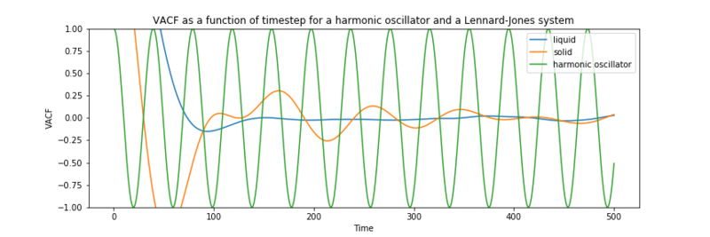
The VACF for a harmonic oscillator (with $\omega =1/2\pi$), calculated using $C\left(\tau \right)=cos\left(\omega \tau \right)$, was plotted against the VACF for the liquid and solid Lennard-Jones systems in figure 18. The most notable difference is regarding the damping of the oscillations: while both the Lennard-Jones solid and liquid oscillations decay for the aforementioned reasons, the harmonic oscillator VACF does not decrease in amplitude since it is an ideal system, with no perturbations disrupting its oscillations.

JC: Be more specific, what are the perturbations? Collisions between particles randomise the velocities and make the VACF decay to zero, there are no collisions in the harmonic oscillator. Look at the equation for the VACF again, when is it negative?

Task 24

Use the trapezium rule to approximate the integral under the velocity autocorrelation function for the solid, liquid, and gas, and use these values to estimate $D$ in each case. You should make a plot of the running integral in each case. Are they as you expect? Repeat this procedure for the VACF data that you were given from the one million atom simulations. What do you think is the largest source of error in your estimates of D from the VACF?

Figure 19. VACF integral versus time for a Lennard-Jones system in vapour, liquid and solid state

Figure 20. VACF integral versus time for a Lennard-Jones system in vapour, liquid and solid state (one million atoms)

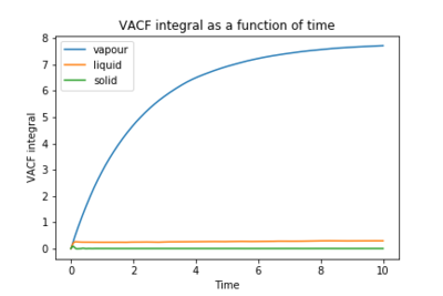
Consistent with the plots of the VACF as a function of time, the graphs of the running integral of the VACF (calculated using scipy.integrate.simps in Python), shown in figures 19-20, are all expected to plateau once the VACF has decayed to 0. This plateau occurs relatively early in the case of liquids and solids, whereas for the vapour case, the integral increases significantly and has not visibly plateaued after $\mathrm{\Delta }t=10$, as expected since the vapour VACF has not completely decayed in this time interval (figures 16-17).

The values of the integrals at t=10 were used as approximations for the plateau value (which represents a good estimate for $\underset{0}{\overset{\mathrm{\infty }}{\int }}⟨\mathbf{v}\left(0\right)\cdot \mathbf{v}\left(\tau \right)⟩\mathrm{d}\tau$) in order to calculate the diffusion coefficient using $D=\frac{1}{3}\underset{0}{\overset{\mathrm{\infty }}{\int }}⟨\mathbf{v}\left(0\right)\cdot \mathbf{v}\left(\tau \right)⟩\mathrm{d}\tau$. The results are shown in table 5 and they are mostly consistent with the values obtained previously by using the MSD (table 4). However, the calculated values for the vapour phase, especially in the case of the one million atoms simulation, are expected to be less accurate since the VACF does not decay completely within the simulated time range, affecting the accuracy of the approximation of the integral. The fact that the running integral plot does not plateau is therefore expected to be the largest source of error in this calculation.

Table 5. Diffusion coefficient calculated using the VACF

Data set	Diffusion coefficient
	Vapour	Liquid	Solid
8000/32000 atoms	2.57	9.79x10-2	-1.14x10-4
1000000 atoms	3.27	9.01x10-2	4.52x10-5

JC: Good, but show the graphs on separate axes so that it's clear that the solid and liquid integrals have reached a plateau. The trapezium rule is another possible source of error.

Conclusion

Simulations under various conditions and in different ensembles were run for Lennard-Jones systems in order to extract a range of data: density versus temperature, heat capacity versus temperature, RDF, MSD and VACF. The obtained results were correlated and compared with theory and with the expected behaviour of real systems. The MSD and VACF data was used to calculate the diffusion coefficient and the obtained values were in accordance with previously reported literature values. The relatively high uncertainty in the results obtained for the diffusion coefficient using the VACF was attributed to the approximations made when calculating the VACF integral.

References

- ↑ J. P. Hansen and L. Verlet, Phys. Rev., 1969, 184, 151-161.
- ↑ P. Atkins and J. Paula, Atkins' Physical chemistry, Oxford University Press, Oxford, 9th edn, 2010.
- ↑ H. Safdari et al., Phys. Rev., 2017, 95, 012120-15.
- ↑ 4.0 4.1 R. L. Rowley and M. M. Painter, Int. J. Thermophys., 1997, 18, 1109-1121.