Talk:Mod:hc02

JC: General comments: Good report on the whole and nicely laid out. Make sure that you understand exactly what system you are simulating so that you can explain the properties and behaviour that you see.

Introduction

The aim of the Year 3 Liquid Simulations Computational Laboratory is to explore computer simulation of chemical systems. Molecular dynamics simulation is a deterministic method used to study the interactions, positions, velocities and forces of complex systems.

Simulations will be performed on the High Performance Computing system at Imperial College London. The software package used is Large-scale Atomic/Molecular Massively Parallel Simulator (LAMMPS). LAMMPS works by simulating and monitoring the classical behaviour of particles. In this laboratory, a simple liquid is being simulated by LAMMPS. To simulate a real system, approximations need to be made as the Schrodinger equation cannot be solved for systems more complicated than a Hydrogen atom. To visualise the data generated from the simulations the software VMD was used. VMD allowed lattice structure, vibrations and motion of the atoms to be visualised.

Within a system, there can be intermolecular and intramolecular interactions. Intermolecular interactions are a combination of the external field, pair potential, three body interactions, the Lennard-Jones potential and coulombic interactions. Intramolecular interactions can be harmonic (for a rigid bond), bending or torsional. In a simple liquid, the molecule can be assumed to behave like a harmonic oscillator with only a Lennard-Jones interactions between molecules.

JC: Harmonic (intramolecular) bonds are not rigid.

Introduction to Molecular Dynamics Simulation

The Classical Particle Approximation - Verlet Algorithm

The velocity-Verlet algorithm can be used to model the behaviour of a classical harmonic oscillator. This method relies on a Taylor expansion to simplify the integration by treating each section discretely, as opposed to continuous treatment; timesteps are used. The Verlet algorithm allows determination of the position of the particle and minimises the error in integration. Using the HO.xls file provided, complete the ANALYTICAL, ERROR and ENERGY columns. The completed file is shown here, HO.xls file.

The ANALYTICAL column gives the classical solution of the position at time, t. The position of a classical harmonic oscillator is given by Equation (1).

$$\begin{gathered} x\left(t\right)=A\cos (\omega t+\varphi ) \\ (1) \end{gathered}$$

The values for A, $\omega$ and $\varphi$are provided in the excel spreadsheet; A = 1.00, $\omega$ = 1.00 and $\varphi$ = 0.00.

This can then be compared against the solution given by the velocity-Verlet algorithm, in column x(t). A plot comparing the positions using the two methods is given in Figure 1. The position of an atom on a harmonic oscillator follows a cosine curve with a minimum of -1.00 and a maximum of +1.00.

Figure 1: The position of the particle at time, t using a classical approach and the velocity-Verlet algorithm.

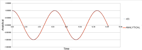
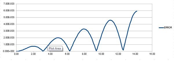
Figure 1 shows that both approaches are appropriate for the harmonic oscillator as it behaves classically, however there is an error associated. The error does not seem to be significant, both methods for determining position are in good agreement. To determine the error, find the modulus of the difference between the velocity-Verlet solution and the classical solution; the modulus is taken because error cannot be negative. Figure 2 shows the calculated error, it is clear that the error increases with time. This is because error is additive so accumulates through time due to the velocity-Verlet algorithm being calculated by a Taylor expansion. By estimating the positions of the local maxima and plotting against time, it can be confirmed that error increases linearly with time. There is a linear line-of-best-fit with an $R^2$ value of 1, this shows there is a perfect fit.

JC: The maximum error increases with time, but the error oscillates rather than increasing monotonically with time, why is this? Is the line of best fit really perfect, what is the R squared value to 3 s.f.?

Figure 2: The error between the classical solution for position and the velocity-Verlet algorithm for position with respect to time.

The total energy of a particle is the sum of the kinetic energy and potential energy; this is shown in Equation (2).

$$\begin{gathered} E=\frac{1}{2}m{v}^2+\frac{1}{2}k{x}^2 \\ (2) \end{gathered}$$

The values for the velocity ($v$) and position ($x$) are given by the velocity-Verlet algorithm, shown in the HO.xls file. Using these values, it is simple to calculate the Energy change with time, Figure 3.

Figure 3: The error between the classical solution for position and the velocity-Verlet algorithm for position with respect to time.

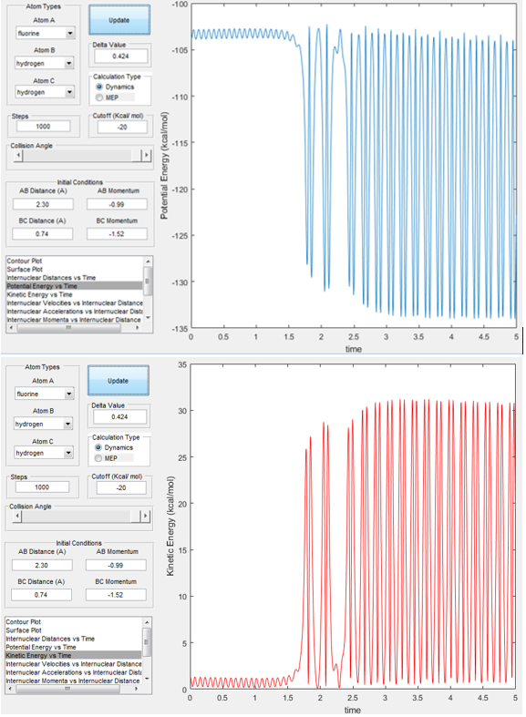
JC: Figure 3 looks like a plot of energy against time from LAMMPS simulations, not the error of the Velocity Verlet harmonic oscillator as the caption says.

The energy conservation law states that the total energy of the system must remain constant.It is important to be able to monitor the total energy of system when modelling its behaviour numerically to ensure the energy conservation law is upheld. Figure 3 shows that energy is relatively constant throughout the simulation with slight oscillations between 0.5 - 0.49887 which can be ignored as the oscillation is small.

The data above, is for a simulation with a timestep of 0.1, the timestep can be changed to give a change in energy of less than 1% over the course of the simulation. For this to be achieved, a timestep of 0.2 needs to be used, this is the critical value. This value was obtained by changing the timestep on the excel document, this resulted in a change in all the values and the plots. Increasing the timestep affected reduces the difference in energy between the maxima and minima; the larger the timestep, the smaller the difference. Increasing the timestep does not only affect the energy, it affects the position and the particle too; as timestep increase the velocity-Verlet approximation becomes a poor approximation of a harmonic oscillator so the error increases.

JC: Choice of timestep of 0.2 is correct, but I think you have uploaded the wrong file for figure 3.

When modelling a system by computer simulation, it is important to measure the energy and error to ensure the results are meaningful.

Lennard-Jones Interaction - Atomic Forces

The Lennard-Jones potential is a approximation of pairwise interactions; attractive and repulsive interactions are summed. The overall Lennard-Jones interaction is given by Equation 3:

$$\begin{gathered} U\left({\mathbf{r}}^N\right)=\sum _i^N\sum _{i\ne j}^N\left\{4ϵ(\frac{{\sigma }^{12}}{r_{ij}^{12}}-\frac{{\sigma }^6}{r_{ij}^6})\right\} \\ (3) \end{gathered}$$

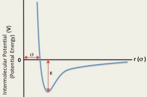
Figure 4: Showing the Potential Energy curve of a Lennard Jones interaction with distance between particles.

A single Lennard-Jones interaction is given by equation 4:

$$\begin{gathered} \varphi \left(r\right)=4ϵ(\frac{{\sigma }^{12}}{r^{12}}-\frac{{\sigma }^6}{r^6}) \\ (4) \end{gathered}$$

The separation, $r_0$ of a single Lennard-Jones interaction at which the potential energy is zero:

1. $0=4ϵ(\frac{{\sigma }^{12}}{r^{12}}-\frac{{\sigma }^6}{r^6})$
2. $0=(\frac{{\sigma }^{12}}{r^{12}}-\frac{{\sigma }^6}{r^6})$
3. $r=\sigma$

Force is given by Equation 5:

$$\begin{gathered} F=\frac{-dU}{dr} \\ (5) \end{gathered}$$

To determine the force of a single Lennard-Jones interaction, differentiate with respect to r to obtain: $F=4ϵ(\frac{-12{\sigma }^{12}}{r^{13}}+\frac{6{\sigma }^6}{r^7})$

As $r=\sigma$when the potential energy is zero:

1. $F=4ϵ(\frac{-12{\sigma }^{12}}{{\sigma }^{13}}+\frac{6{\sigma }^6}{{\sigma }^7})$
2. $F=4ϵ(\frac{-12}{\sigma }+\frac{6}{\sigma })$
3. $F=4ϵ\left(\frac{6}{\sigma }\right)$
4. $F=\frac{24ϵ}{\sigma }$or $F=\frac{24ϵ}{r}$

At the equilibrium separation the force is equal to zero:

1. $0=4ϵ(\frac{-12{\sigma }^{12}}{r^{13}}+\frac{6{\sigma }^6}{r^7})$
2. $0=\frac{-12{\sigma }^{12}}{r^{13}}+\frac{6{\sigma }^6}{r^7}$
3. $\frac{12{\sigma }^{12}}{r^{13}}=\frac{6{\sigma }^6}{r^7}$
4. $r^{-6}=\frac{6{\sigma }^6}{12{\sigma }^{12}}=\frac{1}{2{\sigma }^6}$
5. $r=(\frac{1}{2{\sigma }^6}{)}^{\frac{-1}{6}}=2^{\frac{1}{6}}\sigma$

The well depth is the potential energy. To find the well depth at $r_{eq}$:

1. $\varphi =4ϵ\frac{{\sigma }^{12}}{(2^{\frac{1}{6}}\sigma {)}^{12}}-4ϵ\frac{{\sigma }^6}{(2^{\frac{1}{6}}\sigma {)}^6}$
2. $\varphi =4ϵ\frac{{\sigma }^{12}}{4{\sigma }^{12}}-4ϵ\frac{{\sigma }^6}{2{\sigma }^6}$
3. $\varphi =ϵ-2ϵ$
4. $\varphi =-ϵ$

Evaluation of the integral $\underset{y}{\overset{x}{\int }}\varphi \left(r\right)\mathrm{d}r$ when $\sigma =ϵ=1.0$:

$\underset{y}{\overset{x}{\int }}\varphi \left(r\right)\mathrm{d}r=4[\frac{-1}{11r^{11}}+\frac{1}{5r^5}{]}_y^x$

When $x=\mathrm{\infty }$ and $y=2$

$4[\frac{-1}{11r^{11}}+\frac{1}{5r^5}{]}_2^{\mathrm{\infty }}=0-4(\frac{-1}{11(2^{11})}+\frac{1}{5(2^5)})=-0.0248$

When $x=\mathrm{\infty }$ and $y=2.5\sigma$

$4[\frac{-1}{11r^{11}}+\frac{1}{5r^5}{]}_{2.5}^{\mathrm{\infty }}=0-4(\frac{-1}{11(2.5^{11})}+\frac{1}{5(2.5^5)})=-8.18\text{x}10^{-3}$

When $x=\mathrm{\infty }$ and $y=3\sigma$

$4[\frac{-1}{11r^{11}}+\frac{1}{5r^5}{]}_3^{\mathrm{\infty }}=0-4(\frac{-1}{11(3^{11})}+\frac{1}{5(3^5)})=-3.29\text{x}10^{-3}$

The integration of the Lennard-Jones potential gives the pairwise interaction. From evaluation of the integrals, it is possible to see that as the lower boundary increases the integral increases (becomes less negative but the magnitude decreases. Beyond a certain value of y, the pairwise interaction becomes negligible; by determination of the integral, it is possible to determine this value.

JC: All maths correct and clearly presented.

Periodic Boundary Conditions

Periodic boundary conditions are an approximation for infinitely large systems, by assuming the system is made up of repeating unit cells hence the properties of one unit cell are applicable to the entire system.

The number of water molecules in 1 mL (0.001 L):

1. Convert the volume into mass by multiplying by density; $mass=0.001L\text{x}1000g{L}^{-1}=1g$
2. Convert mass to moles by dividing by the molecular weight; $moles=\frac{1}{18.015gmo{l}^{-1}}=0.0555$
3. Multiply by Avogadros number to obtain the number of molecules; $0.0555\text{x}{N}_A=3.34\text{x}10^{22}$

The volume of 10000 water molecules:

1. Divide by Avogadros number to obtain the moles; $moles=\frac{10000}{N_A}=1.66\text{x}10^{-20}$
2. Convert moles to mass by multiplying by the molecular weight; $mass=1.66\text{x}10^{-20}\text{x}18.015=2.99\text{x}10^{-19}$
3. Convert the mass to volume by dividing by density; $volume=\frac{2.99\text{x}10^{-19}}{1000}=2.99\text{x}10^{-22}L$

Atoms are enclosed in a simulation box to approximate a bulk solution. The box is infinitely repeated in all directions so is very exposed to vacuum.

JC: Using periodic boundary conditions means that the simulation box is not placed in a vacuum.

Consider a cubic simulation box (0, 0, 0) to (1, 1, 1) to which periodic boundary conditions are applied. For an atom at position (0.5, 0.5, 0.5) which moves alone the vector (0.7, 0.6, 0.2), the final position is (0.2, 0.1, 0.7).

JC: All calculations correct.

Reduced Unit Quantities

Distance: $$\begin{gathered} r^{*}=\frac{r}{\sigma } \\ (6) \end{gathered}$$ Energy: $$\begin{gathered} E^{*}=\frac{E}{ϵ} \\ (7) \end{gathered}$$ Temperature: $$\begin{gathered} T^{*}=\frac{k_{B}T}{ϵ} \\ (8) \end{gathered}$$

For Argon, $\sigma =0.34nm,\frac{ϵ}{k_B}=120K$ and $r*=3.2$

• Using Equation 6, $r=3.2\text{x}0.34=1.088nm$
• Using Equation 7, rearrange to $E=\frac{120k_B{N}_A}{1000}=0.997kJmo{l}^{-1}$
• Using Equation 8, $T=\frac{T*ϵ}{k_B}=1.5\text{x}120=180K$

JC: Correct.

Equilibration

Before beginning a simulation, it is important to specify the initial states of all the atoms in the system. The minimum requirement is the starting position of each atom, this is difficult for a liquid because there is no long range order. A potential solution to this would be to use random coordinates for the position of an atom, this does not work. Using random starting coordinates is not a viable solution because, for example, if two atoms are two close together the overlap is large resulting in a large potential energy, this is shown in Figure 4. A strong repulsive interaction occurs due to the high potential energy resulting in the two atoms moving apart at speed. To compensate for the speed of motion of the atoms, a short timestep is necessary. As the atoms are moving away from each other at speed, there is increased rate of collision with other atoms resulting in increased rate of reaction.

To prevent the repulsive force, atoms are placed on the lattice points of a cubic lattice for the course of this experiment. The input file contains the line below, which corresponds to the number spacing. The "sc" component gives the lattice structure and the number gives the number of atoms in the unit cell/the number density.

lattice sc 0.8

In the log file, the line below corresponds to the cubic lattice points, this corresponds to the number density.

lattice spacing in x,y,z = 1.07722 1.07722 1.07722

The number density is the number of lattice points per volume.

1. $V=1.07722^3=1.249$
2. The unit cell contains only one lattice point; $\frac{1}{1.249}=0.8$

For a face-centred cubic lattice (Figure _) with a number density of 1.2:

1. The number of lattice points is 4 so the volume $=\frac{4}{1.2}=3.33$
2. Length of the cube is the cube route of the volume, this gives a result of 1.494 reduced units.
3. For 1 box of length 10, the number of atoms created is 4000. This value is obtained by multiplying the volume (1000) by the number of lattice points in the unit cell (4); 4 x 10 x 10 x 10.

JC: Correct.

In addition to the position of the atoms, the mass, forces and velocity can also be specified.

The following command:

mass 1 1.0
pair_style lj/cut 3.0
pair_coeff * * 1.0 1.0

Definitions:

• Line 1: means the mass of each atom is set from 1 to 1.0.
• Line 2: means use the Lennard-Jones potential with no Coloumbic interactions with a cut-off of the Lennard Jones potential equal to 3.0.
• Line 3: The pairwise force field coefficients for all the atoms are set to 1.0.

JC: The first "1" in the mass command corresponds to atom type 1 (there is only one type of atom in your simulations) and the "1.0" is the mass of atoms of this type. What do the "*" mean in the pair_coeff command?

When we are specifying the position $x_i(0)$ and the velocity $v_i(0)$ of the atom, the velocity-Verlet algorithm for integration can be used because as seen above, it provides a good approximation for the harmonic oscillator model.

JC: If x(0) and v(0) are given as initial conditions, then the Velocity Verlet algorithm is used rather than the standard Verlet algorithm, which requires x(0) and x(-dt) as initial conditions.

To specify a timestep, the following lines are used:

### SPECIFY TIMESTEP ###
variable timestep equal 0.001
variable n_steps equal floor(100/${timestep})
variable n_steps equal floor(100/0.001)
timestep ${timestep}
timestep 0.001

Instead of the lines:

### RUN SIMULATION ###
run ${n_steps}
run 100000

The reason the first code is used over the second code is for ease when needing to change the timestep. The code also ensures simulation occurs at the same time with no dependence on the chosen timestep. This is useful for comparing the effect of timestep on a simulation. This code creates a variable which saves the need to change each value manually as each variable is pre-defined, so by only changing the value of the variable, the value is changed for the runs which follow.

JC: Good explanation.

Checking Equilibration

As thermodynamic properties can be calculated experimentally, it is a useful tool to determine if a simulation if modelling the system correctly. LAMMPS is able to calculate the thermodynamic properties for comparison with the experimental values.

Energy $\delta t=0.001$	Temperature $\delta t=0.001$	Pressure $\delta t=0.001$

Figure 5: Showing the energy, temperature and pressure variation throughout a simulation run at timestep 0.001

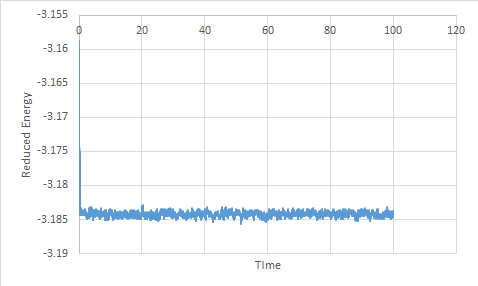
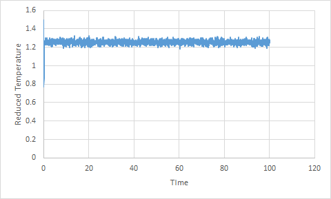
For the timestep 0.001, the energy, temperature and pressure plots show that the system reaches equilibrium; this is known because the average is constant. Each of the thermodynamic properties shows fluctuation due to the assumptions made during the simulation.

Energy	Temperature	Pressure

Figure 6: Showing the affect of varying timestep on the energy, temperature and pressure curves

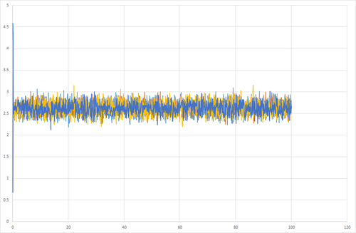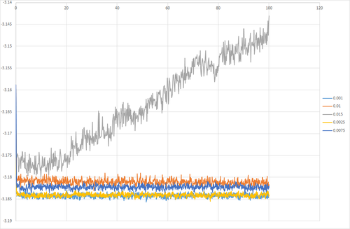
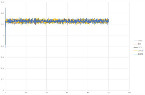
Simulations were run at a range of timesteps to investigate the effect on the thermodynamic properties. It was found that short timesteps provided the best result as equilibrium was reached and the system showed the least fluctuation. At longer timesteps, there was a greater fluctuation so high error. At even longer timesteps, equilibrium was not reached by the end of the simulation. At timestep 0.015, the curve does not plateau, this indicates that the system does not equilibrate. For all the other timesteps investigated, the system is able to reach equilibration. Timesteps 0.001 and 0.0025 have the smallest fluctuations in energy, hence these provide the best results. 0.0025 is chosen over 0.001 because it results in a faster simulation at suitable accuracy.

JC: It is not the size of the energy fluctuations, but the fact that the energy should not depend on the chosen timestep which makes the smallest two timesteps suitable choices.

Running Simulations under Specific Conditions

Changing the conditions of a simulation changes the ensemble. An ensemble contains three properties which must be kept constant, only 3 properties can be maintained as constant at any one time. By changing the ensemble of a reaction means we can gain an understanding of the property on the reactivity.

The equipartition theorem states that every degree of freedom has an energy of $\frac{1}{2}{k}_{B}T$; this relates the temperature of a system with the energy. Degrees of freedom can be defined as ways in which the system is free to change.

Within this system there are 3 degrees of freedom; translational, rotational or vibrational. Electronic transitions are also possible but this is ignored as is generally negligible. The kinetic energy is given by Equation 9.

$$\begin{gathered} \frac{1}{2}\sum _i{m}_i{v}_i^2=\frac{3}{2}N{k}_{B}T \\ (9) \end{gathered}$$

JC: Your system contains spherical particles, so there is no rotational or vibrational motion and electronic transitions are not included because the simulations are classical, they are not just ignored because they are negligible. The three degrees of freedom are due to motion in the x, y and z directions.

There are fluctuations even in parameters which are being maintained. The actual temperature with vary so the temperature which has been input is purely a target, $\mathfrak{𝔗}$. When the actual temperature can be higher or lower than the target, this affects the kinetic energy by a constant scaling factor, $\gamma$. which ensures $T=\mathfrak{𝔗}$.

$\frac{1}{2}\sum _i{m}_i{\left(\gamma v_i\right)}^2=\frac{1}{2}\sum _i{m}_i{\gamma }^2{v}_i^2=\frac{3}{2}N{k}_B\mathfrak{𝔗}$

1. Rewrite: $\frac{3}{2}{\gamma }^{2}N{k}_{b}T=\frac{3}{2}N{k}_b\mathfrak{𝔗}$
2. Cancel terms: ${\gamma }^{2}T=\mathfrak{𝔗}$
3. Rearrange: $\gamma =\sqrt{\frac{\mathfrak{𝔗}}{T}}$

A thermostat ensures the temperature of a system is maintained at a set values. A barostat maintains the pressure of a close system. To change the temperature and pressure of a simulation, variable needs to be changed in the input file.

variable T equal ... #insert temperature
variable p equal ... #insert pressure
variable timestep equal 0.0025

The reduced temperatures chosen to run simulations at are 1.6, 1.6, 1.7, 1.8, 1.9 and 2.0. These temperature are suitable as they are all above the critical temperature of 1.5, this is a requirement because the substance is behaving as a fluid.

The reduced pressures chosen are 2 and 4 as looking at the pressure plot in section [1], the pressure is constant around approximately 2.5. Hence, selecting a value higher and a lower value provides a range of results for comparison.

In this simulation, the fluid is simulated under NVE conditions then under NpT conditions. The result of the simulation output provides values for the pressure, temperature and density (along with errors). The output is compared to the result given by the Ideal Gas Law, Equation 10. Using even more points to determine the curves for the Ideal Gas Curve would give a line with $R^2=1$. The Ideal Gas Law assumes there are no interactions between particles.

JC: Density is inversely proportional to temperature in the ideal gas law, so you won't expect a straight line to give a perfect fit to the data points.

$$\begin{gathered} PV=N{k}_{B}T \\ (10) \end{gathered}$$

To determine the density Equation 10 rearranges to $\frac{N}{V}=\frac{p}{k_{B}T}$ In reduced units $k_B=1$ so this becomes:

$\frac{N}{V}=\frac{p}{T}$

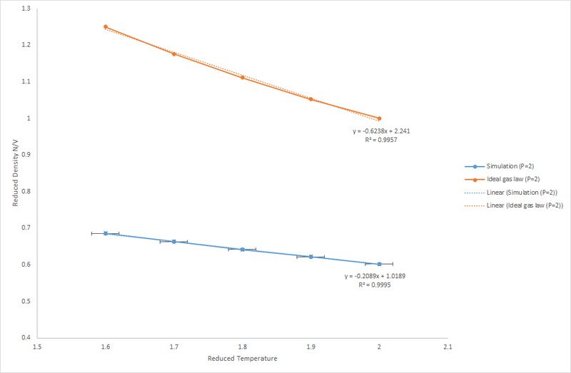
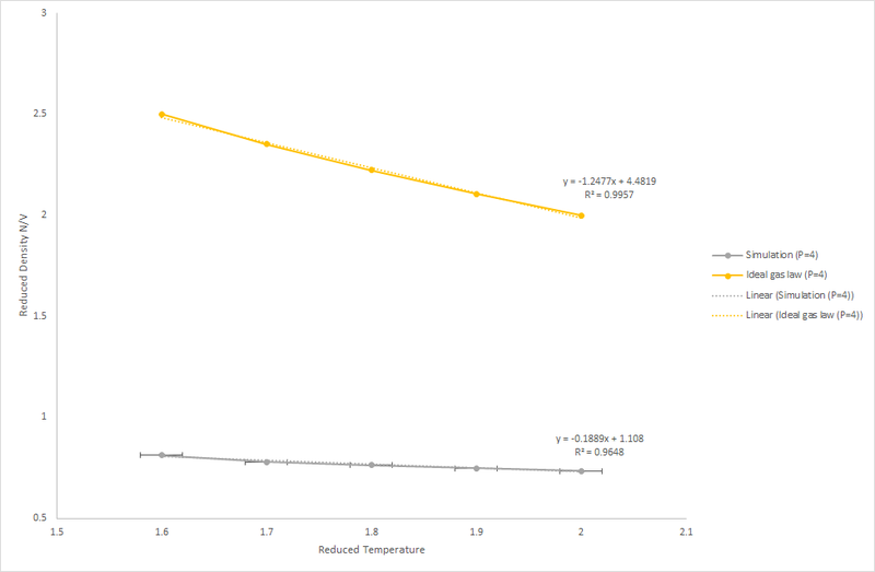
The graphs shown in Figure 7 and 8 show how the density changes with temperature and pressure.

Figure 7: Reduced Density v's Reduced Temperature at P*=2

Figure 8: Reduced Density v's Reduced Temperature at P*=4

As temperature increases the density decreases linearly; the linear relationship is stronger at lower pressure. At higher temperature the fluid has higher kinetic energy resulting in increased motion. Hence, the particle needs to occupy a larger volume to allow more movement, this reduces the density.

As shown in the Ideal Gas Law, there is a direct relationship between the pressure and density. At higher pressures the density of the fluid is significantly higher, this is expected as the density is given by $\frac{N}{V}$ hence at a higher pressure more molecules are occupying a given volume.

The density of the simulations shows a much lower density in comparison to that predicted by the Ideal Gas Law. This indicates that a fluid does not behave ideally; there are pairwise interactions between particles, these can be attractive or repulsive; the fluid is acting like a Lennard-Jones fluid. At higher pressures there is a greater repulsive interaction as the atoms are closer together. Therefore, at higher pressure the gradient is less negative. However, at higher pressures plot of the density according to the ideal gas equation gives a more negative gradient due to the assumption that particles are moving independently of each other so particles can be positioned close together. As pressure is increased, the discrepancy between the ideal gas result and result of the simulation increases.

fix aves all ave/time 100 1000 100000 v_dens v_temp v_press v_dens2 v_temp2 v_press2

The command above calculates the averages for defined variables; density, temperature, pressure, density squared, temperature squared and pressure squared. The values (100 1000 100000) correspond to $N_{every},N_{repeat}$ and $N_{freq}$ respectively. These values give LAMMPS the timesteps and input values necessary to calculate the average of physical properties. The average will be calculated using values sampled every 100 timesteps, 1000 measurements will contribute to the average and an average value will be obtained after 100000 timesteps.

Calculating Heat Capacities Using Statistical Physics

The simulations for this section are calculated in the canonical ensemble; at constant number of atoms, constant volume and constant temperature (NVT). In the canonical ensemble, the heat capacity is the fluctuation in the internal energy with temperature given by Equation 10. The N² term is the number of particles, this is a requirement of LAMMPS.

$$\begin{gathered} C_V=\frac{\partial E}{\partial T}=\frac{\mathrm{V}\mathrm{a}\mathrm{r}\left[E\right]}{k_B{T}^2}=N^2\frac{⟨E^2⟩-{⟨E⟩}^2}{k_B{T}^2} \\ (11) \end{gathered}$$

Input Script:

### DEFINE SIMULATION BOX GEOMETRY ###
lattice sc ... '''#insert density (0.2, 0.8)'''
region box block 0 15 0 15 0 15
create_box 1 box
create_atoms 1 box

### DEFINE PHYSICAL PROPERTIES OF ATOMS ###
mass 1 1.0
pair_style lj/cut/opt 3.0
pair_coeff 1 1 1.0 1.0
neighbor 2.0 bin

### SPECIFY THE REQUIRED THERMODYNAMIC STATE ###
variable T equal ... '''#insert temperature (2.0, 2.2, 2.4, 2.6, 2.8)'''
variable timestep equal 0.0025 #this is the timestep which gave the best results in the quickest time

### ASSIGN ATOMIC VELOCITIES ###
velocity all create ${T} 12345 dist gaussian rot yes mom yes

### SPECIFY ENSEMBLE ###
timestep ${timestep}
fix nve all nve '''#changing the ensemble'''

### THERMODYNAMIC OUTPUT CONTROL ###
thermo_style custom time etotal temp press
thermo 10

### RECORD TRAJECTORY ###
dump traj all custom 1000 output-1 id x y z

### SPECIFY TIMESTEP ###

### RUN SIMULATION TO MELT CRYSTAL ###
run 10000
unfix nve 
reset_timestep 0

### BRING SYSTEM TO REQUIRED STATE ###
variable tdamp equal ${timestep}*100
fix nvt all nvt temp ${T} ${T} ${tdamp} 
run 10000
reset_timestep 0
unfix nvt '''#switching off the thermostat'''
fix nve all nve '''#changing the ensemble'''

### MEASURE SYSTEM STATE ###]
'''#defining variables to use as shortcuts'''
thermo_style custom step etotal temp atoms 
variable etot equal etotal
variable etot2 equal etotal*etotal
variable temp equal temp
variable temp2 equal temp*temp
fix aves all ave/time 100 1000 100000 v_etot v_temp v_etot2 v_temp2
run 100000

variable aveetot equal f_aves[1]
variable aveetot2 equal f_aves[3]
variable avetemp equal f_aves[2]
variable ave2etot equal f_aves[1]*f_aves[1]
variable heatcap equal atoms*atoms*(${aveetot2}-${ave2etot})/(${avetemp}*${avetemp}) '''#using Equation 10, k<sub>B</sub> equals 1'''
variable heatcapvol equal atoms*atoms*((${aveetot2}-${ave2etot})/(${avetemp}*${avetemp}))/vol '''#using Equation 10, k<sub>B</sub> equals 1'''

print "Averages"
print "--------"
print "Temperature: ${avetemp}"
print "heatcap: ${heatcap}"
print "heatcapvol: ${heatcapvol}"

Figure 9: Plot of how the Heat Capacity over Volume changes based on Temperature and Density

JC: Putting a smooth line through the data points is misleading as there is no reason why the heat capacity should follow this line between data points. Equally there is no reason why the trend should be linear.

Figure 9 shows the results of the simulations. The general trend is that Cv/V decreases with increasing temperature; the same trend is observed at both densities. From Equation 11, as the temperature is in the denominator this is the expected trend.

JC: What about the temperature dependence of <E> in the numerator?

Heat capacity is an extensive property so at higher density there is a higher heat capacity. At higher density because there is greater fluctuation because fluctuation is proportional to $\frac{1}{\sqrt{N}}$, hence this is expected. At higher density, the Cv/V is a better fit to a linear line-of-best-fit, this is known as there is a R² value closer to 1. The line-of-best-fit at both densities have the same gradient, this implies that the trend is independent of density.

At higher temperatures the particles have increased kinetic energy, hence want to occupy a larger volume to allow for increased movement. As the density is fixed and the heat capacity decreases with temperature it can be inferred that as there is restricted movement the particles are unable to release and gain energy so reduced fluctuation.

Structural Properties and the Radical Distribution Function

Figure 10: Phase Diagram of a Lennard-Jones Fluid

For all simulation, T = 1.2, this is the critical temperature so the system will not be behaving as a fluid; but the system can behave as a gas, gas and liquid mixture, liquid, liquid and solid mixture or solid. The phase is dependent on the density of the system; gases being the least dense and solids being the most dense. For the solid the structure is a face-centered cubic rather than a standard cubic structure as this results in an increased density. Based on the phase diagram show in Figure 10, the reduced densities selected for a gas, liquid and solid are 0.1, 0,8 and 1.5 respectively.

The Radical Distribution Functions (RDF) were computed using the software VMD then plot using excel. The RDF, FIgure 11, shows the the distribution of particles about a reference particle.

Figure 11: Radial Distribution Functions of a solid, liquid and gas.

For all states, at very short separations the RDF is equal to zero, this is to account for the atomic radius of the particles, they cannot physically be that close.

The coordination number of the first peak:

1. Gas: (1.125, 2.30)
2. Liquid: (1.075, 2.52)
3. Solid (0.95, 5.01)

JC: These are the coordinates of the first peaks, not coordination numbers.

In the gaseous phase, there is a single broad peak. The peak is board because gases are highly disordered systems. A single peak is visible as particles in the gas will position themselves in the most favourable position with maximises the attractive interactions and minimises the repulsive interactions.

Liquids have some degree of order; there is short range order but no long range order. This explains why there are 3 peaks in the RDF, each decreasing in height as distance increases. As there is a higher density, a larger number of particles must occupy the same volume so the RDF closer to the reference is higher than for a gas.

As the solid is the highest density phase, there is a higher population of particles closer to the reference particle. In a solid, as the particles are forced closer together there is the potential for repulsive interactions to minimise this the system needs to be (and is) very ordered. The crystal structure is now a face-centered cube to allow for closer packing of the particles. Due to this order, the RDF plot is uniform with a peak occurring at regular intervals.

For the RDF of the solid, the first three peaks are (0.95, 5.01), (1.35, 1.04) and (1.65, 2.35). The x coordinate corresponds to the position of the particle by giving its distance from the reference. Hence, the first 3 peaks give the distance of the 3 closest particles to the reference.

Figure 12: FCC Crystal Structure

Given that the lattice spacing (LS) is equal to the distance between the reference (R) and atom A; LS = RA = 1.35. Use Figure 12 to prove the distances to the neighbouring atoms and the lattice spacing.

RB is the shortest distance from the Reference (R)

• $RB=\frac{1}{\sqrt{2}}RA=\frac{1}{\sqrt{2}}LS$
• $RB=\frac{1}{\sqrt{2}}1.35$
• $RB=0.95$

RC is the longest distance from R.

• $R{C}^2=R{B}^2+R{A}^2$
• $R{C}^2=0.95^2+1.35^2$
• $RC=1.65$

As RB and RC have been determined, RA can be proved to be 1.35:

• $R{A}^2=R{B}^2+R{B}^2$
• $R{A}^2=2R{B}^2$
• $R{A}^2=2(0.95^2)$
• $RA=1.35$

JC: RB and RC have been calculated assuming RA = 1.35, so it is not surprising that you calculate RA to be 1.35. This is a circular arguement.

Figure 13: Running Integral of the Solid RDF

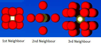
To determine the coordination number, the RDF needs to be integrated, Figure 13. From the plot of the running integral, the plateau's give the coordination number. For the first peak the coordination number is 12. For the second peak the coordination number is 6; subtracting 12 from 18. For the third peak the coordination number is 24; subtracting 18 from 42. This means there are 12 closest neighbouring particles, then 6 second neighbours and 24 third closest neighbours; this is represented in Figure 14.

Figure 14: Nearest Neighbours of a FCC lattice

JC: Good diagram to show the first 3 nearest neighbours.

Dynamical Properties and the Diffusion Coefficient

Mean Squared Displacement

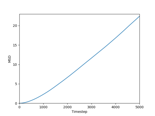
Based on the phase diagram show in Figure 10, the reduced densities selected for a gas, liquid and solid are 0.1, 0,8 and 1.5 respectively. The simulation of each phase gives data which contains the total mean square displacement (MSD), plots of the data are shown in Figure 15. The MSD is a measure of how the position of a particle compared to a reference particle over time.

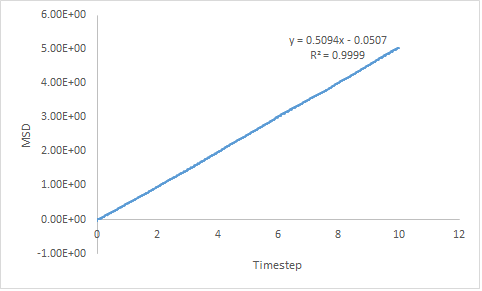
For a gas, the MSD has a linear dependence on time. This is because gases are disordered systems so there is a high extent of motion. Initially, the gas MSD is slightly curved this is because the movement is not random but with time the movement becomes random. The gradient of the curve is higher than that of the liquid because gases are less ordered than liquids, this is mirrored in the MSD with time. The plot of the liquid MSD shows a strong linear fit with an R² close to 1. Liquids show some degree of order.

The MSD of a solid increases rapidly initially as the system establishes a high level of order to form a structure which minimises repulsive interactions. From this initial spike in MSD, the plot plateaus. This is because the system is very ordered so there is no motion.

$$\begin{gathered} D=\frac{1}{6}\frac{\partial ⟨r^2\left(t\right)⟩}{\partial t} \\ (12) \end{gathered}$$

The MSD is connected to the diffusion coefficient, D by Equation 12. Estimated diffusion coefficients are calculated by multiplying the gradient of each plot by $\frac{1}{6}$:

• D_Gas = 1.62
• D_Liq = 0.0849
• D_Sol = 8.33x10^-7

The trend exhibited by the diffusion coefficients is as expected; D_Gas > D_Liq > D_Sol. The more ordered the system, the lower the diffusion coefficient and the slower the rate of diffusion; the inverse is also true. As the gradient of the line-of-best-fit has been used to determine the diffusion coefficient there is a degree of error associated.

Gas	Liquid	Solid

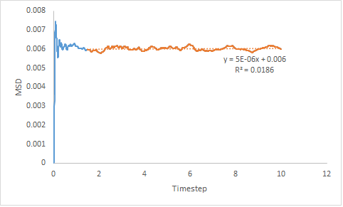Figure 15: Showing the MSD v's Timestep plot of a gas, liquid and solid.

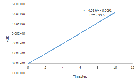
The effect of varying the number of particles in the system is monitored. MSD output files for systems containing a million particles were provided.

For a gaseous system containing one million particles, the line-of-best-fit is a poorer fit compared to that of a smaller system. A reason for this discrepancy is due to differing densities. In the simulation for a smaller system the density input was 0.1; however it is unknown which density was used to simulate the million particle system.

JC: The quality of the line of best fit depends on when you decide that the simulation has reached the linear, diffusive regime.

For the liquid MSD, both plots provide very similar results. This implies that simulation of a larger system is not necessary for a liquid as a reliable result can be produced with a smaller system. This is preferred as it is less computationally demanding.

For the solid MSD for a million particles, the plot shows the same trend as before but the curve is smoother. It is clear that using a large system provides a more reliable line-of-best-fit, this allows for a more accurate diffusion coefficient to be estimated.

Estimated diffusion coefficients are calculated by multiplying the gradient of each plot in Figure 16 by $\frac{1}{6}$:

• D_Gas = 2.97

• D_Liq = 0.0873

• D_Sol = -8.33x10^-6 or 5.00x10^-6

The same trend in the diffusion coefficient is expressed by small and large systems but the estimation is more accurate when determined for a larger system. However, for the solid system the diffusion coefficient obtained using only the linear section of the graph gives a negative gradient, hence negative diffusion coefficient. When the line-of-best-fit of the entire curve is use, a positive value for the diffusion coefficient is obtained. Both methods give a results very close to zero; this is because theoretically the diffusion coefficient for a solid should be zero. Reasons for error are due to assumptions made by LAMMPS or due to the system size so the intervals over which the MSD is measured are larger than for a small system.

Gas	Liquid	Solid

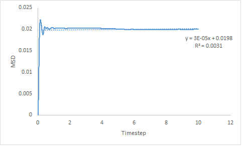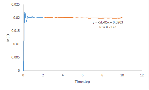Figure 16: Showing the MSD v's Timestep plot of a gas, liquid and solid for a million particles.

Velocity Autocrrelation Function

The Diffusion coefficient can also be calculated using the velocity autocorrelation function, Equation 13. The velocity autocorrelation function, Equation 13, gives the difference in velocity at time $t+\tau$ compared to time $t$

$$\begin{gathered} C(\tau )=<v(t).v(t+\tau )> \\ (13) \end{gathered}$$

For a 1D harmonic oscillator:

1. The position is given by Equation 1.
2. The velocity is the derivative of the position, the differential of Equation 1 needs to be taken: $v=-A\omega sin(\omega t+\varphi )$
3. The normalised velocity autocorrelation function for a 1D harmonic oscillator: $C\left(\tau \right)=\frac{\underset{-\mathrm{\infty }}{\overset{\mathrm{\infty }}{\int }}v\left(t\right)v(t+\tau )\mathrm{d}t}{\underset{-\mathrm{\infty }}{\overset{\mathrm{\infty }}{\int }}{v}^2\left(t\right)\mathrm{d}t}$

Evaluation of $v\left(t\right)v(t+\tau )$

1. $(-A\omega \sin (\omega t+\varphi ))(-A\omega \sin (\omega (t+\tau ))+\varphi )=A^2{\omega }^2\sin (\omega t+\varphi )\sin (\omega t+\varphi +\omega \tau )$
2. Use the trigonometric identity $sin(\alpha +\beta )=sin(\alpha )cos(\beta )+sin(\beta )cos(\alpha )$
3. $v(t)v(t+\tau )=A^2{\omega }^2\sin (\omega t+\varphi )(\sin (\omega t+\varphi )\cos (\omega \tau )+\cos (\omega t+\varphi )\sin (\omega \tau ))$

Evaluation of $v^2(t)$:

1. $(-A\omega \sin (\omega t+\varphi ))(-A\omega \sin (\omega t+\varphi ))$
2. $v^2\left(t\right)=A^2{\omega }^2{\sin }^2(\omega t+\varphi )$

Evaluate: $C(\tau )=\frac{\underset{-\mathrm{\infty }}{\overset{\mathrm{\infty }}{\int }}{A}^2{\omega }^2\sin (\omega t+\varphi )(\sin (\omega t+\varphi )\cos (\omega \tau )+\cos (\omega t+\varphi )\sin (\omega \tau ))\mathrm{d}t}{\underset{-\mathrm{\infty }}{\overset{\mathrm{\infty }}{\int }}{A}^2{\omega }^2{\sin }^2(\omega t+\varphi )\mathrm{d}t}$

1. Cancel the constants A and $\omega$: $C(\tau )=\frac{\underset{-\mathrm{\infty }}{\overset{\mathrm{\infty }}{\int }}\sin (\omega t+\varphi )(\sin (\omega t+\varphi )\cos (\omega \tau )+\cos (\omega t+\varphi )\sin (\omega \tau ))\mathrm{d}t}{\underset{-\mathrm{\infty }}{\overset{\mathrm{\infty }}{\int }}{\sin }^2(\omega t+\varphi )\mathrm{d}t}$
2. Rearrange the fraction to: $C\left(\tau \right)=\frac{\underset{-\mathrm{\infty }}{\overset{\mathrm{\infty }}{\int }}{\sin }^2(\omega t+\varphi )\cos (\omega \tau )\mathrm{d}t}{\underset{-\mathrm{\infty }}{\overset{\mathrm{\infty }}{\int }}{\sin }^2(\omega t+\varphi )\mathrm{d}t}+\frac{\underset{-\mathrm{\infty }}{\overset{\mathrm{\infty }}{\int }}\sin (\omega t+\varphi )\cos (\omega t+\varphi )\sin (\omega \tau )\mathrm{d}t}{\underset{-\mathrm{\infty }}{\overset{\mathrm{\infty }}{\int }}{\sin }^2(\omega t+\varphi )\mathrm{d}t}$
3. Take out the constants: $C\left(\tau \right)=\cos (\omega \tau )\frac{\underset{-\mathrm{\infty }}{\overset{\mathrm{\infty }}{\int }}{\sin }^2(\omega t+\varphi )\mathrm{d}t}{\underset{-\mathrm{\infty }}{\overset{\mathrm{\infty }}{\int }}{\sin }^2(\omega t+\varphi )\mathrm{d}t}+\sin (\omega \tau )\frac{\underset{-\mathrm{\infty }}{\overset{\mathrm{\infty }}{\int }}\sin (\omega t+\varphi )\cos (\omega t+\varphi )\mathrm{d}t}{\underset{-\mathrm{\infty }}{\overset{\mathrm{\infty }}{\int }}{\sin }^2(\omega t+\varphi )\mathrm{d}t}$
4. Cancels the first term and cancel the second term because $sin(\omega t+\varphi )\cos (\omega t+\varphi )=0$ is an asymmetric function:

$C(\tau )=cos(\omega \tau )$

JC: Maths is correct and nicely laid out.

Gas	Liquid	Solid

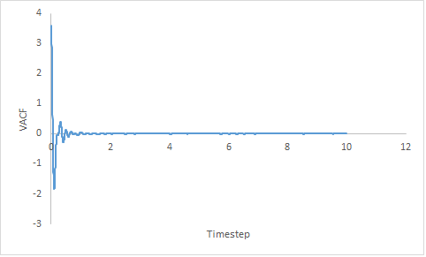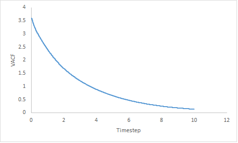
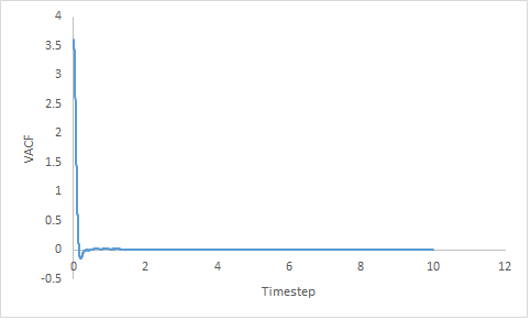
Figure 17: Showing the VACF v's Timestep plot of a gas, liquid and solid for a million particles.

Velocity is directional; the minima in the VACF plots represent a change in the direction of velocity. Changes in direction occur as a result of collision which result in the transfer of energy.

The VACF of a gaseous system decreases gradually; the decrease is slower as the timestep increases. The steadier decrease in velocity is attributed to the disorder of the system. As a gas is low density system; hence it is very unlikely there are any colliding particles as they are far apart.

The VACF of a liquid shows one minima then the curve plateaus at zero. Liquids do not have a high density but collisions can occur with solvent molecules. The hydrogen bonding in liquid water (the solvent) produces an oscillatory motion due to the greater rigidity. Collision with these solvent structures give rise to the single minima.

JC: There is no hydrogen bonding in your system, the collisions are initially with the solvent cage.

The solid VACF shows a large sharp decrease in velocity which then increases to zero with several oscillations. Due to the close packed nature of solids; being in the fcc crystal structure and of high density, there is a high chance of collision.

Overtime, the velocity of a Lennard-Jones system will becomes uncorrelated due to collisions. When the system becomes uncorrelated, the VACF will plateau to zero.

The harmonic oscillator solution fluctuates between C(T) 1 and -1. In a harmonic oscillator, collisions cannot occur as there are no other atoms present, hence the system can never becomes uncorrelated so will never plateau and continues oscillating.

Figure 18: Showing how the VACF plot of a solid and liquid compare to the harmonic oscillator.

The diffusion coefficient can be estimated using Equation 14.

$$\begin{gathered} D=\frac{1}{3}\underset{0}{\overset{\mathrm{\infty }}{\int }}\mathrm{d}\tau ⟨\mathbf{v}\left(0\right)\cdot \mathbf{v}\left(\tau \right)⟩ \\ (14) \end{gathered}$$

The trapezium rule;

$\underset{a}{\overset{b}{\int }}f(x)dx=(b-a)\frac{f(a)+f(b)}{2}$

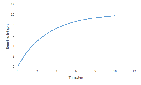
needs to be exploited to estimated the area under the curve. Figure 19 shows the running integral of the MSD curves obtained from the trapezium rule.

Gas	Liquid	Solid

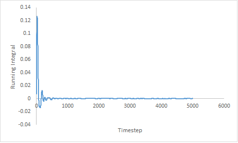Figure 19: Showing the running integral of the VACF curves.

Estimated diffusion coefficients:

• D_Gas = 3.27
• D_Liq = 0.0901
• D_Sol = 4.57x10^-5

Once, again the diffusion coefficients follow the same trend as expected. The estimation of the diffusion coefficient using the VACF method is higher than that predicted from measurement of the MSD. Both estimations of the diffusion coefficient of the liquid are within the same order with an error of 0.28%. The error is negligible and can be assumed to be due to the assumptions made; both methods are considered to be suitable. The estimation of the diffusion coefficient of the solid is more accurate by the MSD method as the value is closest to zero.

Generally, the values of the diffusion coefficient determined by the VACF are larger than those determined by the MSD method. A potential cause of this could be the use of the trapezium rule; using a more sophisticated integration method can give a refined running integral.

JC: Good analysis.