Talk:Mod:hakunamatata

JC: General comments: Good write up with some excellent explanations. Check your spelling and try to write more clearly when explaining your results.

Introduction to Molecular Dynamics Simulations

The Classical Particle Approximation and Numerical Integration

The verit and verit-velocity algorithms are numerical methods to approximate the average position and velocity respectively of randomly moving particles in a particular medium (solid, liquid, fliud etc.). This position and velocity can be applied to Newtonian mechanics to calculate such properties as the force and potential energy of the system. The algorithms work by splitting the function into discrete time steps, calculating the values of position and velocity at this particular time step, and then effectively "joining the dots" to create an approximate function. These simulations always use the answer from the previous timestep to compute the new timestep, so initial conditions must be given for the first step. Both of the algorithms are shown below and are derived from the Taylor expansion of the position or velocity of the atoms at the timestep "n+1" or $t+\delta t$.

Verit Algorithum: ${\mathbf{x}}_i(t+\delta t)\approx 2{\mathbf{x}}_i\left(t\right)-{\mathbf{x}}_i(t-\delta t)+\frac{{\mathbf{F}}_i\left(t\right)}{m_i}\delta t^2$

Verit-Velocity Algorithum:${\mathbf{v}}_i(t+\delta t)={\mathbf{v}}_i(t+\frac{1}{2}\delta t)+\frac{1}{2}{\mathbf{a}}_i(t+\delta t)\delta t$

JC: Be careful with spelling, the algorithm is called the Verlet algorithm.

• ${\mathbf{F}}_i\left(t\right)$ is the force acting on a particular atom as a function of time
• ${\mathbf{a}}_i\left(t\right)$ is the acceleration of the atom at time $t$

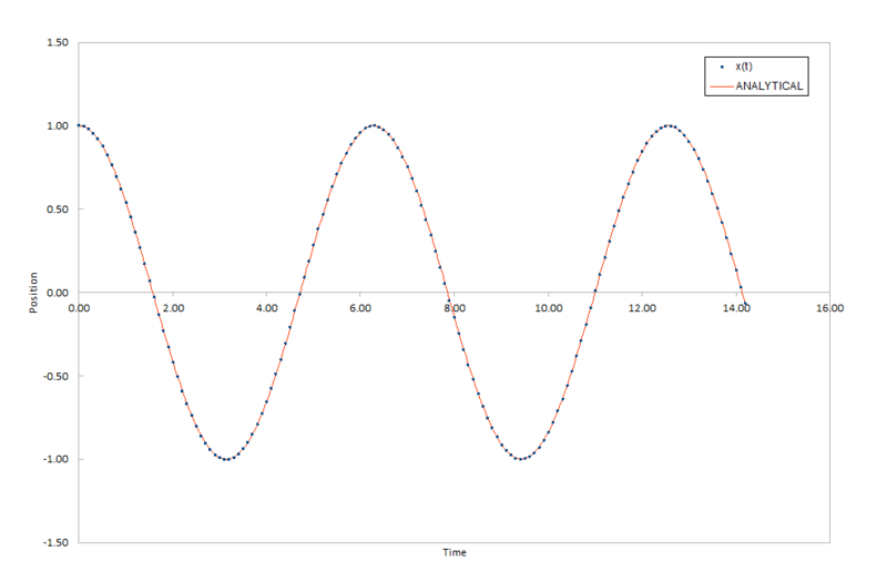
The smaller the timestep, the closer the numerical approximation is to the true function, which can be modeled as a classical harmonic oscillator. Figure 1. in the table below shows the comparison between the two methods at plotting position of an atom as a function of time in time space.

Figure 1. Plots of position vs time comparing the verit algorithm and harmonic spring results	Figure 2. Plot of the total classical energy of the system (potential + kinetic)
The harmonic spring position values are modeled from the harmonic oscillator or particle on a spring. The equation of $x\left(t\right)=A\cos (\omega t+\varphi )$ is used to calculate these values, where $A$ and $\omega$ are equal to 1 and $\varphi$ is equal to zero. As seen on the plot, the curves produced from the two different methods of calculating the position are in good agreement.	The potential energy is calculated using the equation $U=\frac{1}{2}k{x}^2$, with a value of k (force constant) given as 1. The kinetic energy is calculated using the velcity from the verit-velocity algorithm using the equation $T=\frac{1}{2}m{v}^2$, where m (mass) is equal to 1. The total energy of the system, $E$, is equal to $T+U$. The values for $x$ (from the potential energy term) and $v$ (from the kinetic energy term) are taken from the verit algorithm and verit-velocity algorthim respectively.
Figure 3. Plot of the difference (error) between the harmonic spring and verit algorithm data	Figure 4. Plot of the peaks in the error plot in figure 3.
The peaks in the error between the harmonic spring and verit algorithm results are at the point where the position curve crosses the time axis. This is because the harmonic spring data ($x(t)$) has a slightly shorter wavelength than that of the verit velocity algorithm, and therefore the difference will get larger with each period of the wave. This is shown by the error getting larger in figure 3. The period of the plot of the two methods are different because the verit algorithm is much more approximate so does not give the correct solution.	The change in the error/difference between the harmonic spring data and verit algorthm data increases linearly and so therefore period of each of the plots in figure 1. must be constant.

JC: Why does the error plot have an oscillatory shape?

The error can also be quantified on a phase space plot; phase space is momentum or velocity plotted as a function of position. The true solution for motion of an atom is a perfect ellipse, and the more elliptic the shape (less circular) the more momentum or velocity is in the system. A numerical solution, like the verit algorithms, will produce a set of points very close to this ellipse but not perfectly following the curve. A good numerical solution will remain in an elliptical shape, whereas a bad numerical solution, for example one with a large timestep, will spiral away from the true solution. Two examples of such systems using the data from figures a-d are shown below.

Figure 5. Phase plot of the harmonic spring data with a good numerical solution (timestep = 0.1)	Figure 6. Phase plot of the harmonic spring data with a bad numerical solution (timestep = 0.3)

JC: Great extra analysis.

The timestep at which this data is plotted is 0.1, which results in a very small change in the energy, as seen in figure b. Increasing the time step will increase the variation in the energy. To keep the variation in the total energy of the system under 1%, the time step must be no larger than approximately 0.28. The energy varies more with increasing time step because the jumps in the algorithm are getting larger due to less data points. The algorithm assumes these points are joined by a straight line and that the halfway point in the jump is the average between the starting and finishing point of the jump. The phase space plot will become less elliptic and the jumps eventually become so large that the plot is no longer a continuous shape.

JC: What is figure b? Which timesteps did you try to see when the variation in energy goes below 1%?

It is essential to monitor the energy of a numerically modeled system because a good solution for the motion of an atom has a constant energy and a plot in phase space of a perfect ellipse.

Calculating the Interatomic Distance and Force at Zero Potential

From classical mechanics, the force calculated from the Newtonian mechanics above can be used to calculate the potential experienced by an atom in the system. They are related by the equation:

${\mathbf{F}}_i=-\frac{\mathrm{d}U\left({\mathbf{r}}^N\right)}{\mathrm{d}{\mathbf{r}}_i}$

Figure 7. The Lennard-Jones Potential

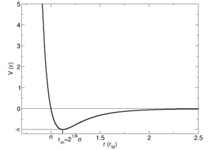
This potential gives the shape and dimension of the potential surface on which the system can be modeled. In this experiment, a simple 1D potential is used to describe the inter atomic forces of a liquid; the Lennard-Jones potential. It has the characteristic features of a short range repulsion potential and harmonic character around the equilibrium bond distance or interatomic separation. The value of $r_0$, the inter atomic separation when the potential, $\varphi \left(r\right)$, is equal to zero, can be calculated by equating the equation for the Lennard-Jones potential to zero and solving for $r$.

The equation for the Lennard-Jones potential: $\varphi \left(r\right)=4ϵ(\frac{{\sigma }^{12}}{r^{12}}-\frac{{\sigma }^6}{r^6})$

Equating this to zero: $0=4ϵ(\frac{{\sigma }^{12}}{r^{12}}-\frac{{\sigma }^6}{r^6})$

And rearranging in order to separate the variables: $\frac{{\sigma }^{12}}{r^{12}}=\frac{{\sigma }^6}{r^6}$

Rearranging this gives $r$ in terms of $\sigma$: $r^6={\sigma }^6$, where $r=r_0$ in this case.

This, therefore, gives the result that interatomic distance at zero potential, $r_0$, is equal to $\sigma$. $\sigma$ in the Lennard-Jones potential is effectively the diameter of one of the particles in the system being measured; in this case, the solid, liquid or gas we are simulating. This is the point where the potential curve crosses the x-axis on an Energy vs interatomic distance plot. The force, ${\mathbf{F}}_i$, at this point on the curve corresponds to the gradient; it is found by calculating the derivative of the curve at this point.

To calculate the force, we must differentiate the equation for the Lennard-Jones potential.

$U\left(r\right)=4ϵ(\frac{{\sigma }^{12}}{r^{12}}-\frac{{\sigma }^6}{r^6})$

$\frac{\mathrm{d}U\left(\mathbf{r}\right)}{\mathrm{d}\mathbf{r}}=-48ϵ{\sigma }^{12}{r}^{-13}+24ϵ{\sigma }^6{r}^{-7}$

As force is equal to the negative differential of the potential energy, the value of the force is: ${\mathbf{F}}_i=48ϵ{\sigma }^{12}{r}^{-13}-24ϵ{\sigma }^6{r}^{-7}$

Substituting in the value of $r$ at zero potential from the calculation before: ${\mathbf{F}}_i=\frac{48ϵ}{\sigma }-\frac{24ϵ}{\sigma }=\frac{24ϵ}{\sigma }$.

The gradient where the Lennard-Jones plot crosses the axis is negative; $ϵ$ in the term obtained for ${\mathbf{F}}_i$ is negative and therefore the overall value of the force will be negative.

Calculating the Interatomic Distance, Force and Well Depth of the Potential at Equilibrium

To calculate the value of $r$ at the equilibrium position, we need to use the derivative of the potential energy curve. The equilibrium value of $r$, $r_{eq}$, is the value at the minimum of the Lennard-Jones curve; when $\frac{\mathrm{d}\varphi \left(\mathbf{r}\right)}{\mathrm{d}\mathbf{r}}=0$.

Therefore, equating the derivative to zero gives: $0=-48ϵ{\sigma }^{12}{r}^{-13}+24ϵ{\sigma }^6{r}^{-7}$

Rearranging this: $48ϵ{\sigma }^{12}{r}^{-13}=24ϵ{\sigma }^6{r}^{-7}$

And simplifying and cancelling gives: $2{\sigma }^6=r_{eq}^6$. Therefore the value of $r$ at equilibrium is: $r_{eq}=\sqrt[6]{2}\sigma$.

Physically, this result means that the equilibrium distance is 1.12 times the diameter of one of the particles; the particles have a small gap between them so do not touch. A short range repulsion potential, as seen in the Lennard-Jones curve, is a result of the particles coming into contact.

Again, the force can be calculated from the derivative of the potential curve at the equilibrium point. As the derivative at this point is zero (a minimum on the curve), the force will therefore also be zero.

The well-depth of the potential curve is the difference between zero potential and the potential at the equilibrium bond length. This can be calculated by substituting the value for the equilibrium bond length into the equation for the Lennard-Jones potential.

$U\left(r\right)=4ϵ(\frac{{\sigma }^{12}}{r^{12}}-\frac{{\sigma }^6}{r^6})$

$U\left(r_{eq}\right)=4ϵ(\frac{{\sigma }^{12}}{4{\sigma }^{12}}-\frac{{\sigma }^6}{2{\sigma }^6})$

Cancelling and simplifying this equation gives: $U\left(r_{eq}\right)=4ϵ\times \frac{1}{4}$

Therefore the absolute value for the well depth is $ϵ$. The actual value of this potential is $-ϵ$, as the equilibrium bond length gives the most stable configuration of the molecules and therefore suggests attractive interactions are involved in the arrangement of the molecules; this attractive potential is negative.

JC: All correct.

Boundary Conditions and the Lennard-Jones Cutoff

When simulating a liquid, it is computationally impractical to simulate a realistic liquid. Therefore a smaller 'box' containing $N$ particles is simulated and the computer program will use periodic boundary conditions to simulate infinite repetitions of this box. For example, when the atom reaches one edge of the box, applying periodic boundary conditions, it will reappear again at the opposite edge of the box as if they were connected. Applying this logic: an atom at the position $(0.5,0.5,0.5)$ in a box of size $(1,1,1)$ moves along the vector $(0.7,0.6,0.2)$. Without periodic boundary conditions, we would assume that the atom would end up at the position $(1.2,1.1,0.7)$. However, in this box, there is no such position and so the particle must reappear at the opposite edge to where it effectively 'left' the box. Therefore, it's ending position will be $(0.2,0.1,0.7)$.

JC: Correct. Periodic boundary conditions are used to remove the interface at the edge of the simulation box and allow bulk properties to be obtained from simulations.

The number of particles, $N$ simulated by the computer is usually between $1000$ and $10000$. Physically, this is a very small volume. Considering water, we can calculate the number of molecules in 1 mL or 1 cm^3, a volume which would be considered small in the lab. Taking the concentration of water at standard conditions, $$\begin{gathered} 55 \\ mol \\ d{m}^{-3} \end{gathered}$$, we can convert it to the number of moles per mL: $$\begin{gathered} 0.055 \\ mol \\ m{L}^{-1} \end{gathered}$$. Multiplying this value by Avagadro's constant ($N_A$) gives the number of molcules of water per mL: $3.02\times 10^{22}m{L}^{-1}$.

The reverse procedure can be used to compare this to the volume of 10,000 molecules: 10,000 divided by Avagadro's constant gives the number of moles of water which 10,000 molecules makes up: $$\begin{gathered} 1.66\times 10^{-20} \\ mol \end{gathered}$$. Dividing this value by the concentration (from $n=cV$, where $n$ is the number of moles, $c$ is the concentration and $V$ is the volume), gives the volume: $$\begin{gathered} 3.02\times 10^{-22} \\ dm \end{gathered}$$ or $$\begin{gathered} 3.02\times 10^{-19} \\ mL \end{gathered}$$. Physically, of course, this is far too small a volume to be recorded in the lab.

Periodic boundary conditions simulate an infinite lattice and therefore, when computing the potential, will calculate an infinite amount of pair interactions. Therefore, it is only practical to calculate the energies up to a certain interatomic distance; the Lennard-Jones cutoff distance. Beyond this point, the potential energy and the integral of the curve beyond this point become insignificant and do not impact on the overall energy; removing interactions beyond this point from the calculations will not effect the accuracy. Multiplying the Lennard-Jones potential with the radial distribution function gives a plot of the probability of finding an atom at a particular interatomic distance. The larger the interatomic distance, the lower the probability and so the energy after the cutoff can be disregarded. The radial distirbution function is dicussed in a later section.

Integrating over the Lennard-Jones curve and applying this cutoff as the lower limit can show how small the integral is:

For a general cutoff of with value $x$:

$I=\underset{x}{\overset{\mathrm{\infty }}{\int }}U\left(r\right)\mathrm{d}r=\underset{x}{\overset{\mathrm{\infty }}{\int }}\frac{4ϵ{\sigma }^{12}}{r^{12}}\mathrm{d}r-\underset{x}{\overset{\mathrm{\infty }}{\int }}\frac{4ϵ{\sigma }^6}{r^6}\mathrm{d}r$

Solving this: $I=4ϵ{\sigma }^{12}{\frac{-1}{11r^{11}}|}_x^{\mathrm{\infty }}-4ϵ{\sigma }^6{\frac{-1}{5r^5}|}_x^{\mathrm{\infty }}$

This gives the general solution: $I=\frac{4ϵ{\sigma }^{12}}{11x^{11}}-\frac{4ϵ{\sigma }^6}{5x^5}$

Evaluating this for $ϵ=\sigma =1$: $I=\frac{4}{11x^{11}}-\frac{4}{5x^5}$

When the cutoff point $x$ is $2\sigma$ (or 2 considering $\sigma =1$): $I=-0.025$

When the cutoff point $x$ is $2.5\sigma$ (or 2.5 considering $\sigma =1$): $I=-0.0082$

When the cutoff point $x$ is $3\sigma$ (or 3 considering $\sigma =1$): $I=-0.0033$

All values are taken to 2 significant figures. As the cutoff value for the interatomic distance gets larger, the integral gets smaller, and therefore the energy excluded from the calculation becomes smaller, and the second term in the solved integral, $I$, dominates the energy value.

JC: Correct.

Reduced Units

When using the Lennard-Jones potential, it is appropriate to use reduced units for intermolecular distance, energy and temperature, which makes the maths and axes of plots much easier to understand. Reduced units can be calculated by the following relationships:

Intermolecular distance: $r^{*}=\frac{r}{\sigma }$, Energy: $E^{*}=\frac{E}{ϵ}$, Temperature: $T^{*}=\frac{k_{B}T}{ϵ}$

$\sigma$ and $ϵ$ are scaling factors. For example, if the parameters for Argon are:

• $\sigma =0.34nm$
• $$\begin{gathered} ϵ \\ / \\ {k}_B=120K \end{gathered}$$
• Lennard-Jones cutoff $r*=3.2$

Then the value of $r$ in real units is $1.088nm$. The well-depth, $ϵ$, is $0.999kJmo{l}^{-1}\approx 1kJmo{l}^{-1}$. The value of $T*=1.5$ in real units is $180K$.

The reduced units in this experiment has $k_B=1$.

All simulation computations are run using the computer program LAMMPS.

JC: Values are correct, but you should only give answers to the same number of significant figures as used in the question (in this case 2).

Equilibration

The first aim of the experiment is to determine the most appropriate timestep, $\delta t$, to use in the verit algorithm simulations. This timestep is a balance between the accuracy of the results (the smaller the timestep, the closer to the true function the result will be) and the length of real time over which the simulation is run (the smaller the timestep, the less real time over which the simulation will give a result). The appropriateness of the timestep will be determined by plotting the total free energy of the simulated lattice as a function of time, and seeing how it equilibrates.

Five different calculations, which simulated the melting of a crystal and subsequent equilibration of the energy of the melted crystal, were run at five different timesteps; 0.001, 0.0025, 0.0075, 0.01 and 0.015. They were described by the NVE or "microcanonical ensemble". An ensemble is a collection of samples of a system which are under three thermodynamic constraints (three properties are kept constant); in the microcanonical ensemble, the number of particles, the volume and the total energy is kept constant (NVE).

These calculations simulate a box of 1000 unit cells and use periodic boundary conditions to replicate the simulation to a larger scale. Because these simulations use the numerical methods defined in the previous section, the initial position and velocity of the atoms must be defined in the input file. The Brownian (uncorrelated, random) motion of the atoms in the simulation means that there is no long range order in the system and so the atoms in a real system would start in random positions. However, assigning random starting coordinates to the atoms in a simulated liquid is not a relative process; the coordinates are generate independently of each other. Therefore there is a probability that the coordinates simulated will cause the atoms to overlap, which would give a very large repulsion potential, as seen in the Lennard-Jones potential at very small interatomic distances. This short-range repulsion potential comes from the hard-sphere atomic repulsion model.

JC: A simulation starting from a configuration with high repulsion is likely to be unstable and to crash unless a much smaller timestep is used.

The input file also defines the structure and density of the lattice. The number density of lattice points in any lattice is the number of lattice points per volume of the unit cell. In a simple cubic lattice, there is one lattice point in the unit cell. From an sc lattice with a lattice spacing (length of one side of the unit cell) of $1.07722$, the number density of the lattice points is calculated by:

$\frac{N}{V}=\frac{1}{1.07722^3}=0.7999\approx 0.8$

In a face-centered cubic lattice (fcc), there are four lattice points in the unit cell. Rearranging the above relationship, the lattice spacing can be calculated from the number of lattice points in a unit cell and number density, $1.2$:

$$\begin{gathered} Lattice \\ spacing=\sqrt[3]{\frac{number \\ of \\ lattice \\ points \\ per \\ unit \\ cell}{number \\ density}}=\sqrt[3]{\frac{4}{1.2}}=1.49 \end{gathered}$$

The simulation creates a 3D box which includes 1000 unit cells; 10 unit cells in each dimension. For a simple cubic lattice, because there is one lattice point per unit cell, there will be 1000 atoms created as seen in the input file. The create_atom command in the input file determines how many boxes are created in the simulation and therefore how determines many atoms will be created. If a face centered cubic lattice is simulated, as there are 4 lattice points per unit cell, 4000 atoms will be created by the create_atom command.

The input script also contains the following commands which defines the potential surface which is used to model the intermolecular reactions:

mass 1 1.0

This instruction sets the mass type for the atoms being simulated. It takes the general form of “mass I value”, where mass is the keyword which tells LAMMPS what the input is, I is the atom type and value is the mass of the atom. In this case, I is defined by a specific numerical value; 1 as there is only 1 type of atom in the simulation, but it could be defined with an asterisk (1*), which means “all atom types of 1 to n inclusive” if there are n types of atoms in the simulation.

pair_style lj/cut 3.0

This instruction sets the type of potential which LAMMPS uses in its calculation of pairwise interactions. It takes the general form of “pair_style style args”, where pair_style is the keyword for LAMMPS, style defines the potential and any specifications it may have, and args are the arguments required for this particular potential. In this case, the Lennard-Jones potential has been used (lj) with a cutoff point (cut) of 3σ. The cutoff point is explained in the introduction section.

pair_coeff * * 1.0 1.0

This instruction specifies the coefficients for the pairwise interactions of each pair of atoms, and it takes the general form “pair_coeff I J args”. Pair_coeff is the keyword, I and J are the atom types, and args are the coefficients which the different atoms types take. In this case, the asterisk in place of I and J refers to all atoms types from 1 to n. The coefficients are the pairwise interactions are 1 for each atom, meaning each atom has an equal contribution to the interaction.

JC: For a Lennard-Jones potential, the pair coefficients are the values sigma and epsilon for the interaction between two atoms types. What is sigma and epsilon in this case?

In these initial calculations, the initial conditions for the numerical methods, $x_i(0)$ and $v_i(0)$ are specified. For this experiment, the verit-velocity algorithm would be the most appropriate, as both the starting position and velocity is specified for this algorithm.

To define the timestep for the algorithm the following code is used defining the timestep as a variable instead of just giving it a definite value

### SPECIFY TIMESTEP ###
variable timestep equal 0.001
variable n_steps equal floor(100/${timestep})
variable n_steps equal floor(100/0.001)
timestep ${timestep}
timestep 0.001

### RUN SIMULATION ###
 run ${n_steps}
 run 100000

It is much easier to use the variable version of defining the timestep because the length of time over which the simulation is run depends on the time step. By using a variable, the length of the simulation is kept the same, no matter the size of the timestep. It also makes it easier if multiple properties depend on the timestep – only the variable needs to be changed, not all the parts of the script where timestep is defined.

JC: Correct.

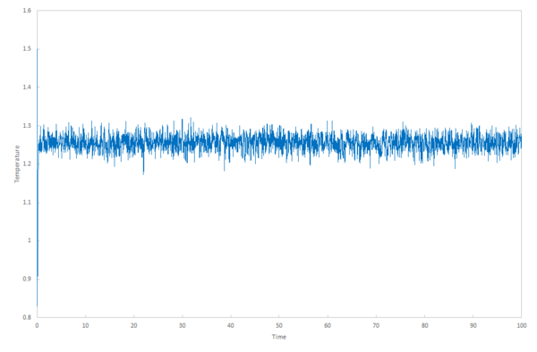
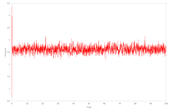
The calculations produce the values for the total energy of the system, temperature and pressure in the output files, which can be plotted against time. How well these values equilibrate determines the appropriateness of the timestep to use in further calculations in the experiment.

Figure 8. Plot of the equilibration of total energy for five different timesteps	Figure 9. Plot of the temperature vs time equilibration for timestep = 0.0025	Figure 9. Plot of the pressure vs time equilibration for timestep = 0.0025

The largest time step to give an acceptable result is 0.01. However, for any simluation we would expect energy to be independent of the timestep, something which is not true at a timestep greater than 0.0025. Therefore, the most appropriate timestep to use for a balance between accuracy and length of time which the simulation covers is 0.0025.

0.015 is a particularly bad choice of timestep. This is because the verit-velocity algorithm gives only an approximate result to the velocity (kinetic energy term) and position (potential energy term), and so when the timestep becomes too large with respect to the time, the algorithm no longer becomes a suitable way to calculate the energy. As seen in the graph of 0.015, the energy does not equilibrate and diverges.

The plots for temperature and pressure vs time give a good indication of an appropriate pressure and temperature to use for running the simulations under specific conditions in the next section .

JC: Good choice of timestep and explanation.

Running Simulations Under Specific Conditions

The calculations in this section are run in the isobaric-isothermal ensemble, where the number of particles in the system, the pressure and the temperature are kept constant (NpT). This means that the temperature and the pressure are recalculated in every step, so are no longer constant like they were in the NVE ensemble. From the equipartition theorem, each degree of freedom will contribute $\frac{1}{2}{k}_{B}T$ of energy to the system. As the system is in three dimensions, there are three degrees of translational freedom and so the total internal energy is equal to $\frac{3}{2}{k}_{B}T$. Equating this to the kinetic energy, $\frac{1}{2}\sum _i{m}_i{v}_i^2$, at the end of every step and rearranging will allow calculation of the temperature after every step.

A target temperature, $\mathfrak{𝔗}$, is defined in the input script. The system will equilibrate by multiplying the velocity by a factor, $\gamma$, in order to accommodate for fluctuations in the overall velocity. This keeps the system at approximately the target temperature and therefore a constant internal energy. If the temperature of the system is greater than the target temperature, the system's kinetic energy is too high, so $\gamma$ is reduced to compensate for this. The same is true for is the temperature is lower than the target temperature; $\gamma$ must be greater than one in the next step to increase the kinetic energy which is now too low. The principle is the same for controlling the pressure.

$\gamma$ can be derived from equating the kinetic and internal energy of the system at an arbitrary time step:

$\frac{1}{2}\sum _i{m}_i{\left(\gamma v_i\right)}^2=\frac{3}{2}N{k}_B\mathfrak{𝔗}$

Expanding the brackets inside the sum and moving the term containing $\gamma$ out of the sum: $\frac{{\gamma }^2}{2}\sum _i{m}_i{\left(v_i\right)}^2=\frac{3}{2}N{k}_B\mathfrak{𝔗}$

As $\frac{1}{2}\sum _i{m}_i{v}_i^2=\frac{3}{2}N{k}_{B}T$, we can replace $\frac{1}{2}\sum _i{m}_i{v}_i^2$ on the left hand side of the equation with $\frac{3}{2}N{k}_{B}T$: $\frac{3{\gamma }^2}{2}N{k}_{B}T=\frac{3}{2}N{k}_B\mathfrak{𝔗}$

Simplifying and rearranging for $\gamma$, gives: $\gamma =\sqrt{\frac{\mathfrak{𝔗}}{T}}$

JC: Derivation is correct, however, there is no need to write down in words what you are doing at each step and it might be slightly easier to follow if you just include the maths.

As temperature and pressure are no longer constant, the input files require specification of the pressure and the temperature for each of the systems which are simulated. 10 simulations were run at two different pressures with five different temperatures at each pressure.

• Temperatures: 1.6, 1.9, 2.2, 2.5, 2.8
• Pressures: 2.5, 3.0

These pressures were chosen because the data simulated when choosing an appropriate timestep gave a pressure between 2.5 and 3.0 (figures 8 and 9).

For the code which computes the thermodynamic potentials, this particular line defines how many steps contribute towards the average of the thermodynamic parameters computed in the calculation:

fix aves all ave/time 100 1000 100000 v_dens v_temp v_press v_dens2 v_temp2 v_press2

fix is the keyword, aves is the name of the group of fixes which in this case is the average of the thermodynamic values, all specifies the atoms which the fix is applied to which in this case is all the atoms in the simulated system and ave/time means that compute global time averages are calculated. The following three numbers have the following meaning:

• 100 = use the input values every 100 timesteps
• 1000 = use input values 1000 times for calculating the average
• 100000 = calculate the average every 100000 timesteps

Therefore for the total calculation, which lasts for 100,000 steps, the average will only be calculated once. Assuming 1 value is calculated every timestep, there will be 100,000/100 = 1000 values.

The density data from all ten calculation was plotted on the same graph, along with the density for an "ideal" gas. This density can be derived from the ideal gas law:

$PV=N{k}_{B}T$

Rearranging in terms of density: $\frac{N}{V}=\frac{P}{k_{B}T}$

As these simulations are being run under reduced units, we can take $k_B=1$, and so the density of the ideal gas becomes:

$\frac{N}{V}=\frac{P}{T}$

Therefore, the density of the ideal gas is plotted as the pressure divided by the temperature in pressure-temperature phase space.

Figure 11. Plot of the variation in density with temperature at a defined pressure for the numerically simulated and ideal systems

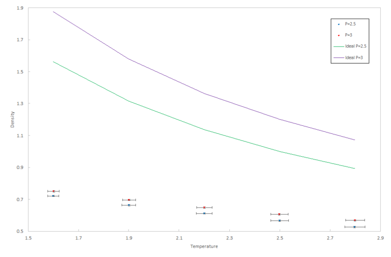
JC: Why have you plotted the ideal gas line with straight lines between data points? You know the analytical function for the relationship between the density and temperature for an ideal gas.

The simulated density is lower than that calculated in the ideal gas law. This is because for an ideal gas, an assumption is made that there are no intermolecular interactions, and therefore forces such as electron repulsion forces are ignored; repulsion forces dominate over attractive ones, as all the atoms in this simulation are the same and so partial charges or dipoles are created. This will mean that the particles move closer together than a real gas and so the density will be larger. This discrepancy between the ideal and non-ideal systems becomes larger at a higher pressure because with a higher pressure, the atoms in the system are closer together and therefore the intermolecular repulsion will become larger. This greater repulsion will in turn have a larger effect on decreasing the density.

JC: Your simulations are completely classical and there are no partial charges or instantaneous dipoles. Repulsion is just due to the Lennard-Jones potential. How does the discrepancy between the ideal gas and your simulations change with temperature?

Statistical Physics Calculations of the Heat Capacity

The heat capacity of a system at constant volume can be calculated from the variance in the total energy of the system. The relationship used to calculate the heat capacity is:

$C_V=\frac{\partial E}{\partial T}=N^2\frac{⟨E^2⟩-{⟨E⟩}^2}{k_B{T}^2}$

$⟨E^2⟩$ is the continuous average of the total square energy at each temperature as a function of temperature. ${⟨E⟩}^2$ is the continuous average of the total energy at each temperature as a function of temperature squared. The heat capacity is multiplied by $N^2$ in this case because the version of LAMMPS calculates every energy divided by the number of molecules in the system simulated.

The calculations in this sections are run in density-temperature phase space and the ensemble has changed to the canonical ensemble (NVT). A set of input files were written for ten calculations for, like the previous section, two pressures and five different temperatures at each pressure:

• Pressure: 0.2, 0.8
• Temperatures: 2.0, 2.2, 2.4, 2.6 and 2.8

$\frac{C_V}{V}$ was plotted against temperature to determine the relationship in density-temperature phase space. An example of an input file can be found here. The lines which have been changed from the previous input files are at the end of the script:

### MEASURE SYSTEM STATE ###

thermo_style custom step etotal temp
variable energy equal etotal
variable energy2 equal etotal*etotal
variable temp equal temp
fix aves all ave/time 100 1000 100000 v_energy v_energy2 v_temp
run 100000

variable aveenergy equal f_aves[1]
variable aveenergy2 equal f_aves[2]
variable avetemp equal f_aves[3]
variable heatcapacitydv equal atoms*atoms*(v_aveenergy2-v_aveenergy*v_aveenergy)/(v_avetemp*v_avetemp*vol)

print "Averages"
print "--------"
print "Temperature: ${avetemp}"
print "Heat Capacity per Volume: ${heatcapacitydv}"

The line with the keyword 'fix' determines which thermodynamic values are averaged and over how many steps they are averaged. The next section takes these averages as variables and uses them to define the heat capacity which is calculated from the equation at the beginning of this section. Only the energy and temperature are needed to define the heat capacity and so only these values are calculated by the simulation.

Figure 12. C_v/V against temperature for the two different pressures 0.2 and 0.8

As seen in figure 11., the heat capacity decreases with temperature for both pressures. It would be expected for an ideal system that as the temperature increases, the heat capacity at constant volume increases and tends to a constant value at very high T of

$3R$

;

$R$

= the universal gas constant. This means increasing the temperature increases the amount of energy being stored in the system and this energy is stored as vibrational energy. However, for a Lennard-Jones liquid, the system being simulated here, the heat capacity decreases with temperature. This is because there are two components to the simulation; the atoms are vibrating in a quasi-harmonic fashion around the equilibrium position and also, they diffuse between neighbouring equilibrium positions in a gas like fashion. As the temperature increases, the amount of diffusion increases and the amount of vibrations decrease, therefore decreasing the ability of the system to take in heat as vibrational energy, resulting in the decrease in heat capacity.

JC: Good research from the literature and good explanation for the trend with temperature. Can you explain how heat capacity changes with density as well?

Structural Properties and the Radial Distribution Function

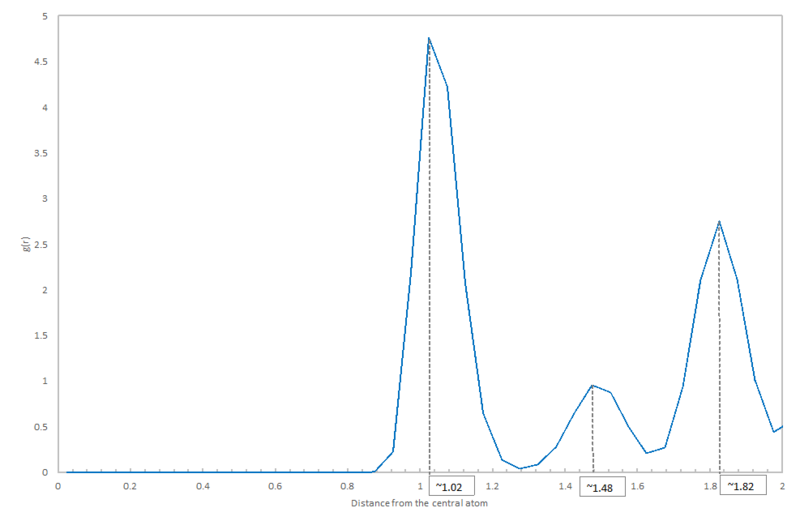
The radial distribution function of a single atom in a system is a plot of the probability that an atom can be found at a certain distance from the central atom. The peaks in this plot gives the distance of an atom from its nearest neighbours in the Lennard-Jones simulated system.

The calculations in this section simulate a Lennard-Jones solid, liquid and gas and, using the output of the LAMMPS trajectory file, plots both the radial distribution function and its integral using DLV. The temperature and pressure parameters for these calculations were taken from the phase diagram or coexistence curve for a Lennard-Jones system. The parameters used are displayed in the table below.

	Temperature, $T^{*}$	Pressure, $p^{*}$
LJ Solid	1.5	1.2
LJ Liquid	1.1	0.8
LJ Gas	1.1	0.01

The data obtained from the plots and the radial distribution functions and their integrals were plotted and shown in the table below.

Figure 13. The radial distribution function (g(r)) plots for a Lennard-Jones solid, liquid and gas	Figure 14. The integrals of the radial distribution function (g(r)) plots for a Lennard-Jones solid, liquid and gas

Figure 15. Representation of a cross section of the first three shells of nearest neighbours in an fcc solid. The black atom is the central atom being considered, the blue atoms are the first shell, the orange atoms the second shell and the purple atoms are the third.

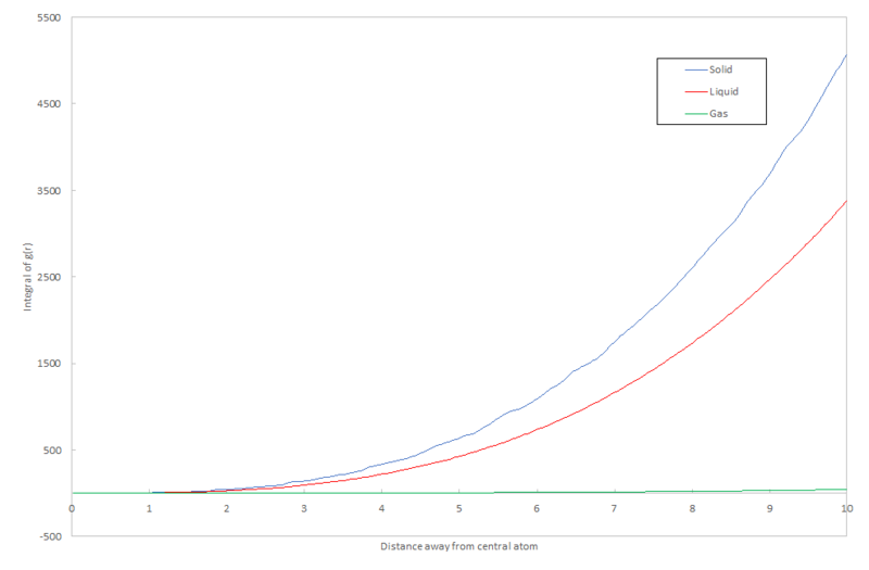
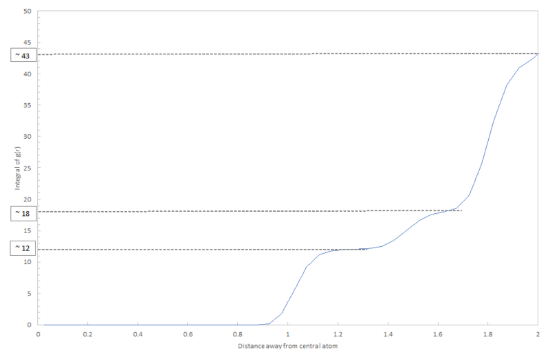
The RDF of the solid gives a very irregular curve because of the irregular structure of the lattice. For a simple cubic lattice, a regular structure of the RDF would be expected because of the equal number of atoms in each of the nearest neighbour shells. However, for face-centered cubic lattice, the solid in this simulation, the structure is much more irregular and as the atoms move from their equilibrium position in the lattice due to vibrations, the peaks in the radial distribution will broaden. The irregular heights of the peaks are due to the varying numbers of atoms in each of the nearest neighbour shells for the central atom. The first shell gives the highest peak as it contains the most atoms multiplied by the strongest interaction potential; in total, considering all four surrounding unit cells, this shell contains 12 atoms and ideally takes the geometry of an icosahedron. The second shell is smaller and contains only 6 atoms in an octahedral coordination shape. The following shell again contributes 12 atoms, 3 from each unit cell. This therefore explains why the heights of the peaks in the solid plot in figure 12. vary. These values can be confirmed by the plot in figure 15. which is the integral; it cumulatively adds the numbers in each shell. The size of the first "step" is 12; there are 12 atoms in the first shell. The size of the second step is approximately 18; there are 18-12=6 steps in the second shell. The same theory applies for the third shell which gives a value of 13. This is slightly different to the predicted value possibly due to error in the calculation of the radial distribution function and therefore its integral.

JC: The solid lattice is not irregular, it is a regular fcc lattice and even for a simple cubic lattice you do not get equal numbers of atoms in the nearest neighbour shells. Good description of the nearest neighbour shells though.

The RDF of the liquid has a representation of far fewer shells, which means that there are less atoms in the space close to a "central" atom in the bulk solution. The particles have more energy and therefore do not keep to a regular lattice structure. As they move about, some regularity is maintained around each atom, but only to the extend of two or three shells, meaning there is no long range order in a Lennard-Jones liquid.

The RDF of the gas again omits more shells as there is almost no order in a Lennard-Jones gas. The single peak on this plot considers only the set of atoms closest to the central atom and all others are disregarded as they are too far apart.

Considering figure 13., the size of the integral of the radial distribution function decreases from solid to liquid to gas. This makes sense as the number of atoms in the surrounding shells decreases with density of the system; the atoms become further apart.

From the plot of the radial distribution function of the solid, the lattice spacing can be determined. For this, we can consider just the first three peaks of the RDF plot. The lattice spacing refers to the length of one unit cell, and so, using figure m, we can calculate this using two different methods; a) we can use the distance between the central atom and the first shell of nearest neighbours, and use trigonometry to calculate the lattice spacing. Or alternatively b) we can use the distance between the central atom and the second nearest neighbour shell to get the lattice spacing.

Figure 16. The radial distribution function (g(r)) plots for the first three peaks of a Lennard-Jones solid	Figure 17. The integral of the radial distribution function (g(r)) plots for the first three peaks of a Lennard-Jones solid

JC: To get the number of nearest neighbours responsible for a particular peak in the RDF, you should take the value of the running integral up until the minimum in the RDF after that peak. If you do this for the 3rd peak peak, you should be looking at the running integral at about r=1.97, which should give a number of nearest neighbours of 42, rather than 43.

Using method a) (with $r$ as the distance between the central atom and the nearest neighbour: Lattice spacing = $\frac{r}{cos(\frac{\pi }{4})}=\frac{1.02}{cos(\frac{\pi }{4})}\approx 1.44$

Using method b): Lattice spacing $\approx 1.48$

We can take an average between the two get an approximate value for the lattice spacing $$\begin{gathered} \approx \\ 1.46 \end{gathered}$$.

JC: Good idea to take an average. How does this value compare with the lattice spacing of the original fcc lattice that the simulation starts with?

These values for distance are all in reduced units.

Dynamical Properties and the Diffusion Coefficient

The ability of atoms to move around in a solid liquid or gas can be characterised by the diffusion coefficient, $D$. In this section, we will explore two different ways to calculate the diffusion coefficient and compare the results.

The Mean Squared Displacement

The diffusion coefficient can be measured easily be calculating the mean squared displacement of atoms in the solution; the diffusion coefficient is proportional to the first derivative of the mean squared displacement. By plotting the mean squared displacement as a function of time, the gradient can be taken to calculate the diffusion coefficient when its has equilibrated and become linear.

The temperature and density parameters used were the same as in the previous section:

• Solid: T=1.5, D=1.2
• Liquid: T=1.1, D=0.8
• Gas: T=1.1, D=0.01

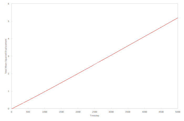
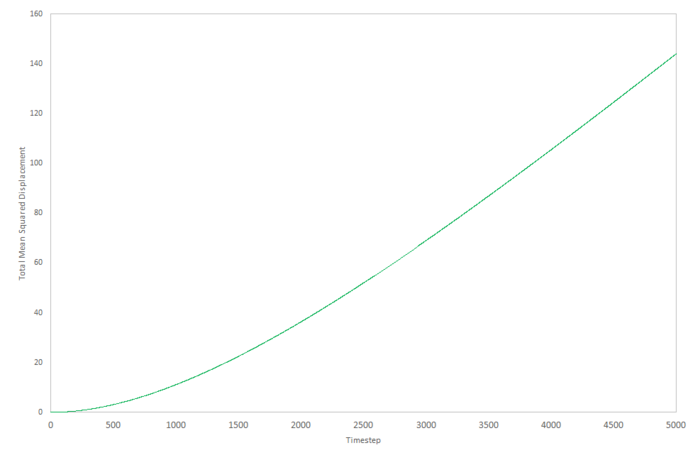
Mean density squared calculations for 8,000 atoms were run for all three Lennard-Jones phases and the data plotted as function of timestep below. The data from a simulation containing 1,000,000 atoms was plotted for comparision.

	Plots for the 8,000 atom data (figures 18-20)	Plots for the 1,000,000 atom data (figures 21-23)
Lennard-Jones solid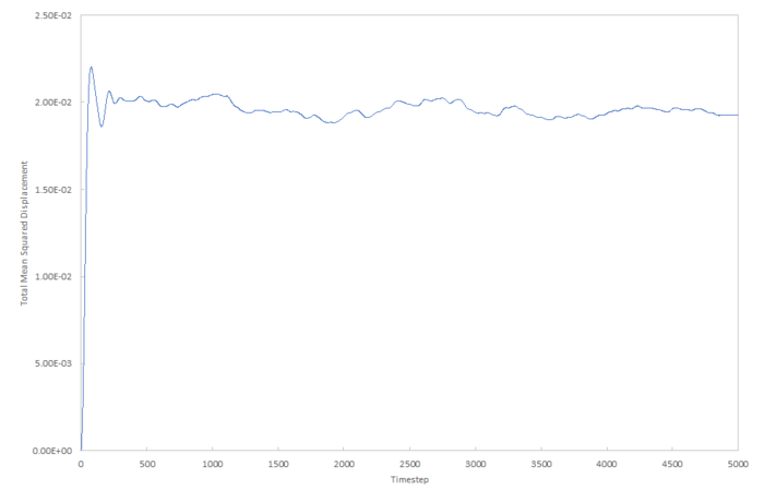
Lennard-Jones liquid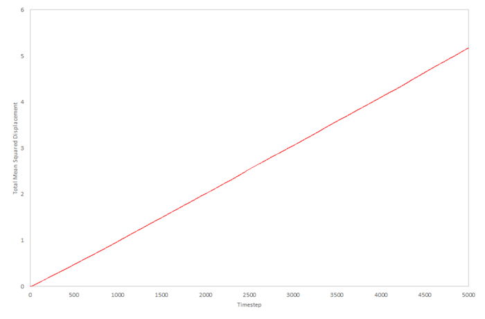
Lennard-Jones gas

The exact relationship between the mean squared displacement and the diffusion coefficient is:

$D=\frac{1}{6}\frac{\partial ⟨r^2\left(t\right)⟩}{\partial t}$

Taking the gradients of each of the curves at the point at which they become linear and dividing by six will give the diffusion coefficient for each set of data. The gradient also needs to be converted to a function of time; this is done by dividing by the timestep, which in this case is 0.002:

	8,000 atom data diffusion coefficients, $$\begin{gathered} D \\ /s^{-1} \end{gathered}$$	1,000,000 atom data diffusion coefficients $$\begin{gathered} D \\ /s^{-1} \end{gathered}$$
Lennard-Jones solid	Gradient $\approx 0$ $D\approx \mathbf{0}$	Gradient $\approx 0$ $D\approx \mathbf{0}$
Lennard-Jones liquid	Timestep corrected gradient = $0.0915$ Amount of data used to calculate gradient: timestep 2500-5000, $R^2=0.9999$ $D=\frac{0.55}{6}=\mathbf{0}\mathbf{.}\mathbf{0}\mathbf{9}\mathbf{1}\mathbf{5}$	Timestep corrected gradient = $0.0915$ Amount of data used to calculate gradient: timestep 2500-5000, $R^2=1$ $D=\frac{0.55}{6}=\mathbf{0}\mathbf{.}\mathbf{0}\mathbf{9}\mathbf{1}\mathbf{5}$
Lennard-Jones gas	Gradient = 0.0972 Amount of data used to calculate gradient: timestep 4300-5000, $R^2=0.9998$ $D=\frac{48.6}{6}=\mathbf{8}\mathbf{.}\mathbf{1}$	Gradient = 0.0386 Amount of data used to calculate gradient: timestep 4000-5000, $R^2=0.1$ $D=\frac{19.6}{6}=\mathbf{3}\mathbf{.}\mathbf{2}$

JC: Good consideration of units when calculating the diffusion coefficients.

For both of the solid approximations, the diffusion coefficient can be approximated as zero. This is because, when equilibrated, the function has a constant value of around 0.2 for the mean squared displacement. A gradient with a value of zero means that the atoms take an infinite amount of time to change their mean squared displacement or move away from their equilibrium position, and so this means that we can approximate in this system, there will be no diffusion. In real system, however, this is not the case; diffusion occurs but it is very slow. A plot for a real system will give a very shallow positive gradient.

The liquid approximations are very well correlated. This is because in both cases, the mean squared displacement of particles in a liquid increases linearly with time and the gradient of both plots are almost identical. We can assume from this that identical starting conditions for temperature and pressure were used to calculate this data. Also, we can estimate that 8,000 atoms is a large enough simulation to give an accurate result for the diffusion coefficient for the Lennard-Jones liquid.

The gas approximations are very different. This is most probably due to the fact that the density specified in each of the calculations is different. The 8,000 data can be estimated to be a much lower density because the diffusion coefficient is faster and this means diffusion will happen faster; at a higher density a particle will take longer to diffuse over a given distance. Because of the difference in density, the two values of the diffusion coefficient cannot be qualitatively compared. The reason for the initial deviation for linearity in the gas plots is due to the momentum of the particles initially dominating over the diffusion and the diffusion coefficient is dependent on time. As the system equilibrates, the diffusion coefficient becomes constant and the plots become linear.

JC: Good comparison of results between the small and large systems.

The Velocity Autocorrelation Function

Another way to calculate the diffusion coefficient is by using the velocity correlation function, which determines how the velocity of an atom changes with time. The function determines the time when the velocity becomes uncorrelated ($\tau$), i.e. the difference between the velocity at time $t$ and at time $t+\tau$. By integrating over this function, we can find the diffusion coefficient.

The velocity autocorrelation function: $C\left(\tau \right)=⟨\mathbf{v}\left(t\right)\cdot \mathbf{v}(t+\tau )⟩$

It can also be written as the integral: $C\left(\tau \right)=\frac{\underset{-\mathrm{\infty }}{\overset{\mathrm{\infty }}{\int }}v\left(t\right)v(t+\tau )\mathrm{d}t}{\underset{-\mathrm{\infty }}{\overset{\mathrm{\infty }}{\int }}{v}^2\left(t\right)\mathrm{d}t}$

Using the function which defines the position of a classical harmonic oscillator, we can differentiate this to give the equation for the velocity which we can plug into the integral:

$x(t)=Acos(\omega t+\varphi )$

$dvx(t)t=v(t)=-A\omega sin(\omega t+\varphi )$

Also needed for the integral:

$v(t+\tau )=-A\omega sin(\omega (t+\tau )+\varphi )$

$v^2(t)=A^2{\omega }^{2}si{n}^2(\omega t+\tau )$

Putting all this into the integral to find the diffusion coefficient:

$C\left(\tau \right)=\frac{\underset{-\mathrm{\infty }}{\overset{\mathrm{\infty }}{\int }}A\omega sin(\omega t+\varphi )\times A\omega sin(\omega (t+\tau )+\varphi )\mathrm{d}t}{\underset{-\mathrm{\infty }}{\overset{\mathrm{\infty }}{\int }}{A}^2{\omega }^{2}si{n}^2(\omega t+\tau )\mathrm{d}t}$

$A^2{\omega }^2$ can be take out of each of the integrals and cancelled. A substituion can then be made to make solving the integral much simpler:

$a=\omega t+\varphi$, $b=\omega \tau$

Therefore, the integral becomes:

$C\left(\tau \right)=\frac{\underset{-\mathrm{\infty }}{\overset{\mathrm{\infty }}{\int }}sin(a)\times sin(a+b)\mathrm{d}t}{\underset{-\mathrm{\infty }}{\overset{\mathrm{\infty }}{\int }}si{n}^2(a)\mathrm{d}t}$

Using the compound angle rule $sin(a+b)=sin(a)cos(b)+cos(a)sin(b)$, the integral can be simplified to:

$C\left(\tau \right)=\frac{\underset{-\mathrm{\infty }}{\overset{\mathrm{\infty }}{\int }}sin(a)sin(a)cos(b)+sin(a)cos(a)sin(b)\mathrm{d}t}{\underset{-\mathrm{\infty }}{\overset{\mathrm{\infty }}{\int }}si{n}^2(a)\mathrm{d}t}$

Separating out into two integrals:

$C\left(\tau \right)=cos(b)\frac{\underset{-\mathrm{\infty }}{\overset{\mathrm{\infty }}{\int }}si{n}^2(a)\mathrm{d}t}{\underset{-\mathrm{\infty }}{\overset{\mathrm{\infty }}{\int }}si{n}^2(a)\mathrm{d}t}+sin(b)\frac{\underset{-\mathrm{\infty }}{\overset{\mathrm{\infty }}{\int }}sin(a)cos(a)\mathrm{d}t}{\underset{-\mathrm{\infty }}{\overset{\mathrm{\infty }}{\int }}si{n}^2(a)\mathrm{d}t}$

$=cos(b)+sin(b)\frac{\underset{-\mathrm{\infty }}{\overset{\mathrm{\infty }}{\int }}sin(a)cos(a)\mathrm{d}t}{\underset{-\mathrm{\infty }}{\overset{\mathrm{\infty }}{\int }}si{n}^2(a)\mathrm{d}t}$

Using the rule $sin(a)cos(a)=\frac{1}{2}sin(2a)$

$C\left(\tau \right)=cos(b)+sin(b)\frac{\underset{-\mathrm{\infty }}{\overset{\mathrm{\infty }}{\int }}\frac{1}{2}(sin(2a))\mathrm{d}t}{\underset{-\mathrm{\infty }}{\overset{\mathrm{\infty }}{\int }}si{n}^2(a)\mathrm{d}t}$

Because the function $\frac{1}{2}sin(2a)$ is symmetric over all space, the second term in this equation becomes zero. Therefore, the integral simplifies to:

JC: The function sin(x) is not symmetric, but antisymmetric or odd, however, you are right that the integral of sin(x) (an odd function) is zero if the limits of the integration are symmetric about x=0

$C\left(\tau \right)=cos(b)=cos(\omega \tau )$

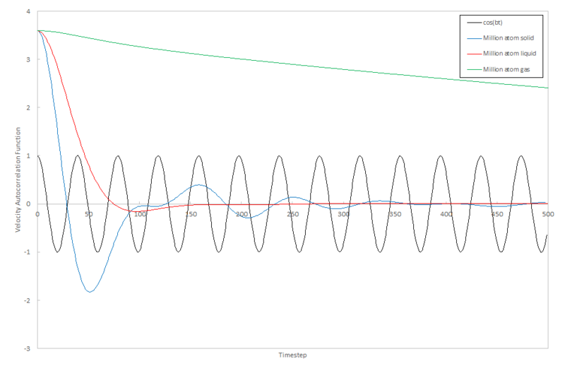
The same calculations from the mean squared displacement section gave an output of the velocity autocorrelation function. The function for the Lennard-Jones solid, liquid and gas were plotted against the timestep along with the approximate function for the velocity autocorrelation function, $cos(\omega \tau )$, where $\omega =\frac{1}{2\pi }$

Figure 24. Plots for the velocity autocorrelation function of a Lennard-Jones solid, liquid and gas; 8,000 atoms	Figure 25. Plots for the velocity autocorrelation function of a Lennard-Jones solid, liquid and gas, 1,000,000 atoms

The plots for the velocity autocorrelation function show how the time correlation of velocity decreases with time due to collisions with other atoms in the system. The Lennard-Jones solid oscillates around the VACF=0 axis with the oscillations becoming progressively more damped with time. The long range of the oscillations is due to the order in the system. Every time the plot crosses the VACF=0 axis, the velocity of the atom changes direction which is due to a collision with another atom. Every collision for every atom is completely uncorrelated so the change in velocity of one atom as it collides is independent of another change in velocity of another colliding atom. Overall, momentum must be conserved and so overall change of velocity in the system must be conserved.

The Lennard-Jones liquid oscillations are damped much quicker; an atom in the liquid only collides with one atom before the velocity becomes uncorrelated with respect to time. The Lennard-Jones gas never reaches the VACF=0 axis as the atoms are too far apart to collide. Because the velocity autocorrelation function never equilibrates, using this method to calculate the diffusion coefficient is inaccurate because the particles in the gas never come into contact with each other.

JC: There are some collisions in the gas which cause a slight decrease in the VACF, however, the frequency of these collisions is much less than in the liquid.

The harmonic oscillating system is so different to the Lennard-Jones systems because the atoms remain in their equilibrium position and vibrate around the same position, never coming into contact with another atom. Because of this, the correlation with time never decreases so the function infinitely oscillates as a sine function.

The diffusion coefficient is calculated from: $D=\frac{1}{3}\underset{0}{\overset{\mathrm{\infty }}{\int }}C\left(\tau \right)\mathrm{d}\tau$

Therefore, the approximate value for the diffusion coefficient using the velocity autocorrelation function is $D=\frac{1}{3}cos(\omega \tau )$

JC: The integral is missing from this expression and the expression only applies to the harmonic oscillator VACF.

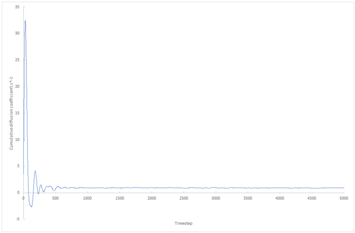
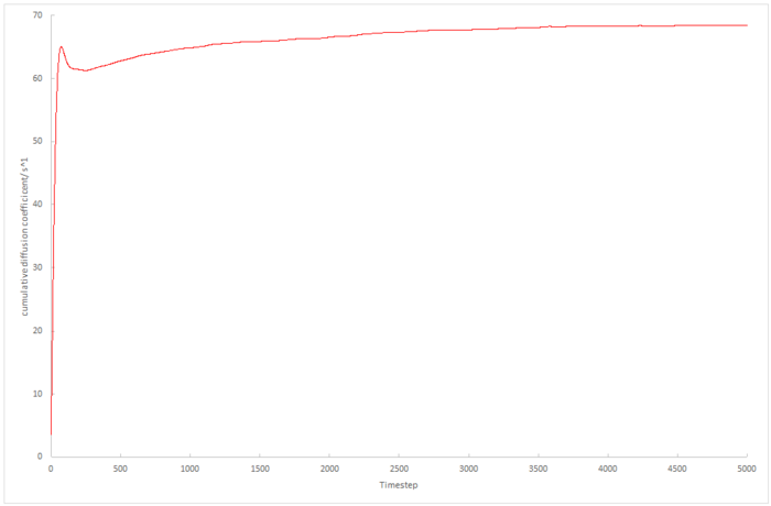
The running integral of the velocity autocorrelation functions was plotted using the trapesium rule, and so the final value on the integral plot is proportional to the diffusion coefficient.

	8,000 atom VACF integral (figures 26-28)	1,000,000 VACF integral (figures 29-31)
Lennard-Jones solid
Lennard-Jones liquid
Lennard-Jones gas

The diffusion coefficients for each of the plots above are tabulated below using the final data point from the integral plot. This is the integral over the whole graph using the trapesium rule. This must be corrected for the timestep; the value is multiplied by 0.002.

	8,000 atom data diffusion coefficients, $$\begin{gathered} D \\ /s^{-1} \end{gathered}$$	1,000,000 atom data diffusion coefficients $$\begin{gathered} D \\ /s^{-1} \end{gathered}$$
Lennard-Jones solid	Timestep corrected integral = $-0.00055$ $D=\frac{-0.00055}{6}=-0.00018\approx \mathbf{0}$	Timestep corrected integral = $0.00014$ $D=\frac{0.00014}{6}=0.000046\approx \mathbf{0}$
Lennard-Jones liquid	Timestep corrected integral = $0.242$ $D=\frac{0.242}{6}=\mathbf{0}\mathbf{.}\mathbf{0}\mathbf{8}\mathbf{0}\mathbf{7}$	Timestep corrected integral = $0.270$ $D=\frac{0.270}{6}=\mathbf{0}\mathbf{.}\mathbf{0}\mathbf{9}\mathbf{0}\mathbf{1}$
Lennard-Jones gas	Timestep corrected integral = $25.6$ $D=\frac{25.6}{6}=\mathbf{8}\mathbf{.}\mathbf{5}\mathbf{5}$	Timestep corrected integral = $9.81$ $D=\frac{9.81}{6}=\mathbf{3}\mathbf{.}\mathbf{2}\mathbf{7}$

The biggest source of error in these plots is that we assume both the 8,000 atom data and the 1,000,000 atom data take the same amount of time to converge. Figure z. shows that 5000 timesteps is not long enough for the velocity autocorrelation coefficient for 8,000 atoms to converge as far as 1,000,000 atom data does in this length of time. As the molecular dynamics simulations simulate random motion, this could induce fluctuations in the velocity autocorrelation plot which could increase or decrease the integral introduction another source of error.

JC: What about the error from using the trapezium rule?

Again, the diffusion coefficient of the Lennard-Jones solid can be assumed to be zero for the same reason as the mean squared displacement data. The diffusion coefficient of the liquid is lower for both sets of data when calculated using the velocity autocorrelation function, and the diffusion coefficient is higher for both sets of data.

JC: This last sentence doesn't make sense.

Summary

A simple Lennard-Jones liquid was simulated for different temperatures, pressures and densities at an optimised timestep of 0.0025. It was found that density of a system decreases with temperature due to particles increasing their kinetic energy and therefore the particles move further apart. The density of an ideal gas is much higher than that of the simulated Lennard-Jones potentials because of lack of repulsive interatomic forces.

It was also found that heat capacity of a Lennard-Jones liquid decreases with increasing temperature, and heat capacity is lower at a lower density. This is due to diffusion dominating atomic vibrations as temperature increases and so ability of a system to absorb heat as vibrational energy decreases with temperature.

It was also found that the radial distribution function and its integral can be plotted to calculate the lattice spacing of a Lennard-Jones solid and the amount of atoms in each nearest neighbour shell respectively. The lattice spacing was calculated as $$\begin{gathered} \approx \\ 1.46 \end{gathered}$$.

The diffusion coefficient for a Lennard-Jones solid, liquid and gas can be calculate using the mean squared displacement or the velocity autocorrelation function. The velocity autocorrelation function was found to be a less reliable method for the gas because the function does not converge in the amount of timesteps that were calculated.

References

- ↑ Dima Bolmatov, V. V. Brazhkin, and K. Trachenko "Thermodynamic behaviour of supercritical matter", Scientific Reports 4 2331 (2013)