Talk:Mod:gogle14

JC: General comments: All tasks attempted and results look good, but some of the written explanations are a bit unclear. Make sure that you understand the background theory behind each task and use this in your answers.

Introduction to molecular dynamics simulations

Analysis of velocity-Verlet integration method

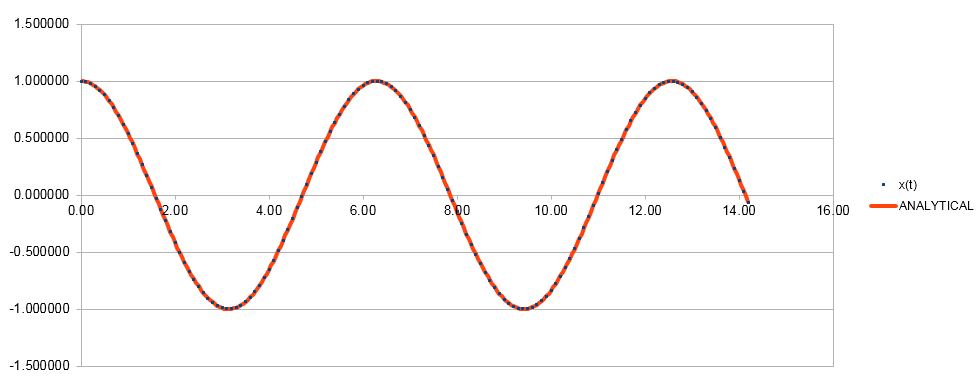
The Verlet algorithm can be used to estimate positions, velocities and momenta of particles without the need of continuous integration. Instead, it uses the knowledge of those values at previous points and Taylor expansion to find all of these values at set intervals (timesteps). Below is a comparison of the function $x(t)=A\cos (\omega t+\varphi )$, where $A=1,\omega =1$ and $\varphi =0$, therefore the function is $x(t)=\cos t$

Figure 1. Comparison of veloity-Verlet and analytical solution of the function.

As can be seen from Figure 1, the results generated by Verlet algorithm match the analytical values closely, indicating how powerful this approximation is.

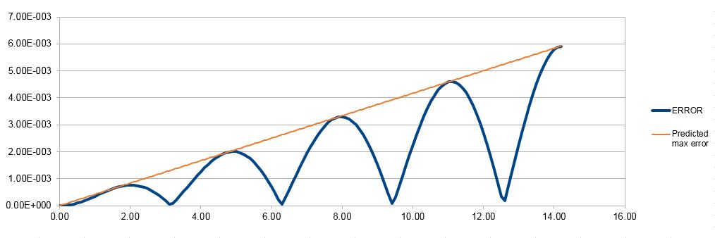
Still, there is some discrepancy present, as indicated in Figure 2 below:

Figure 2. Error analysis for the velocity-Verlet solution.

It can be seen that the error shows an oscillating behaviour (Figure 2), with the local maximum of the error growing consistently over time. This is due to the fact that the Taylor series converge to the real value, but not all terms were taken into account; the first maximum occurs where the fourth term (error term) is the largest. As previous values are used to calculate those at the next timestep, the error is cumulative and therefore increases over time, as predicted by the curve in the graph.

JC: Why does the error oscillate?

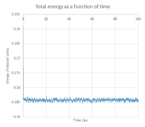
Figure 3. Total energy as a function of time for velocity-Verlet method.

Another way of evaluating the usefulness of this algorithm is by seeing how well the predicted values match known values. As an isolated system is modelled, the total energy in the system should remain constant. However, Figure 3 shows that this is not the case and there are small (0.25%) fluctuations from the real value when the timestep of 0.1 is used. This shows that the system, though faithful, is still a simplification of reality, furthermore, it can tolerate even a larger timestep and thus fewer calculations, as 1% error is exceeded only when the timestep is increased to 0.2. This could save computational resources, but it also indicates the balance between the choice of timestep and the correspondence of the model to reality.

JC: Good.

Evaluation of the system used

$\varphi (r)=4ϵ(\frac{{\sigma }^{12}}{r^{12}}-\frac{{\sigma }^6}{r^6})$

$0=4ϵ(\frac{{\sigma }^{12}}{r_0^{12}}-\frac{{\sigma }^6}{r_0^6})$

$0=(\frac{{\sigma }^{12}}{r_0^{12}}-\frac{{\sigma }^6}{r_0^6})$, multiply by $\frac{r_0^6}{{\sigma }^6}$

$0=\frac{{\sigma }^6}{r_0^6}-1$

$\frac{{\sigma }^6}{r_0^6}=1$

$r_0^6={\sigma }^6$

$r_0=+\sigma$ $or$ $r_0=-\sigma$ (root invalid, as separation has to >0)

This is the separation at which potential energy is 0; the force at this separation is as shown below:

$F=-\frac{d\varphi (r)}{dr}$

and

$\varphi (r)=4ϵ(\frac{{\sigma }^{12}}{r^{12}}-\frac{{\sigma }^6}{r^6})$

therefore,

$F(r_0)=-\frac{4ϵ(\frac{{\sigma }^{12}}{r_0^{12}}-\frac{{\sigma }^6}{r_0^6})}{dr}$

$F(r_0)=-4ϵ(-12\frac{{\sigma }^{12}}{r_0^{13}}+6\frac{{\sigma }^6}{r_0^7})$

$F(r_0)=48ϵ\frac{{\sigma }^{12}}{r_0^{13}}-24ϵ\frac{{\sigma }^6}{r_0^7}$

As we know that $r_0=\sigma$:

$F(r_0)=\frac{48ϵ}{\sigma }-\frac{24ϵ}{\sigma }=\frac{24ϵ}{\sigma }$

A system is said to be an equilibrium when there is no net force acting on it, i.e., the force is 0. By substituting minimum potential energy expression from above into the minimum force expression, the following formula is obtained:

$F_{eq}=48ϵ\frac{{\sigma }^{12}}{r_{eq}^{13}}-24ϵ\frac{{\sigma }^6}{r_{eq}^7}=0$, divide by $24ϵ\frac{{\sigma }^6}{r_{eq}^7}$ and rearrange:

$r_{eq}^6=2{\sigma }^6$

$r_{eq}=+\sqrt[6]{2}\sigma \approx 1.122\sigma$ or $r_{eq}=-\sqrt[6]{2}\sigma \approx -1.122\sigma$ (root invalid, separation has to be >0)

The depth of well characterises how stable the system is. For the equilibrium distance it can be found by substituting the equilibrium $r_0$ value into the Lennard-Jones interaction equation:

$\varphi (r_{eq})=4ϵ(\frac{{\sigma }^{12}}{(\sqrt[6]{2}\sigma {)}^{12}}-\frac{{\sigma }^6}{(\sqrt[6]{2}\sigma {)}^6})=4ϵ(\frac{1}{4}-\frac{1}{2})=4ϵ(-\frac{1}{4})=-ϵ$

To evaluate the integral of the potential energy of the Lennard-Jones potential, let us set the changing lower bound to a value n, which can later be substituted for the necessary value:

$\underset{n}{\overset{\mathrm{\infty }}{\int }}\varphi (r)dr=\underset{n}{\overset{\mathrm{\infty }}{\int }}4ϵ(\frac{{\sigma }^{12}}{r^{12}}-\frac{{\sigma }^6}{r^6})dr$

$ϵ=\sigma =1$, therefore:

$\underset{n}{\overset{\mathrm{\infty }}{\int }}4(\frac{1}{r^{12}}-\frac{1}{r^6})dr=$ $4[\frac{1}{5r^5}-\frac{1}{11r^{11}}{]}_n^{\mathrm{\infty }}=$ $4([0]-(\frac{1}{5n^5}-\frac{1}{11n^{11}}\left)\right)=$ $4(\frac{1}{11n^{11}}-\frac{1}{5n^5})\approx -\frac{4}{5n^5}$, as first term becomes negligible

Let us substitute in the lower bound values ($\sigma$ is still 1):

When $n=2\sigma$, the value is $-0.0248$

When $n=2.5\sigma$, the value is $-0.0082$

When $n=3\sigma$, the value is $-0.0033$

In order to understand the scale of the system, let us compare the number of water particles in 1 mL of water to the volume of water that could be simulated. The number of water particles in 1 mL of water under standard conditions can be determined like this $m=\rho \times V=0.9982\times 1=0.9982(g)$

$n=\frac{m}{N}=\frac{0.9982}{18.02}=5.539\times 10^{-2}(mol)$

$N=n\times N_A=5.539\times 10^{-2}\times 6.023\times 10^{23}=3.336\times 10^{22}$

Meanwhile, 10000 molecules of water occupy this volume:

$n=\frac{N}{N_A}=\frac{10000}{6.023\times 10^{23}}=1.660\times 10^{-20}(mol)$

$m=n\times M=18.02\times 1.660\times 10^{-20}=2.989\times 10^{-19}(g)$

$V=m\times \rho =2.989\times 10^{-19}\times 0.9982=2.983\times 10^{-19}(mL)$

From these results it can be seen that the volumes simulated are absolutely minuscule: 18 orders of magnitude less than a single mL of water. However, even such small amounts are enough to provide us with values applicable to the macroscopic world.

The system also uses boundary conditions in order to ensure that the simulated environment is close to reality while also being easy to simulate $(0.5,0.5,0.5)+(0.7,0.6,0.2)=(1.2,1.1,0.7)$, which is $(0.2,0.1,0.7)$ after applying boundary conditions according to which each atom regenerates at the opposite into the cube each time it crosses its boundaries; no coordinate can exceed 1.

These simulations also make use of reduced units. It is done purely out of convenience so that the output and input could be as close to easily operable numbers while also having a physical meaning. For example, conversion from reduced to real units for Argon can be achieved as follows:

1)Lennard-Jones cutoff distance of 3.2 units

$r=r*\sigma =3.2\times 3.4\times 10^{-10}=1.09\times 10^{-9}(m)$

2)Well depth

$$\begin{gathered} E_{well}=-ϵ=120\times k_b\times N_A=120\times R=120\times 8.31=998(J \\ mo{l}^{-1})=0.998(kJ \\ mo{l}^{-1}) \end{gathered}$$

3)Temperature of 1.5 reduced units

$T=\frac{ϵT*}{k_B}=1.5\times 120=180(K)$

JC: All maths correct and well laid out.

Equilibriation

A randomly generated grouping of atoms can (and, with a large number of generated atoms, likely will) occupy thermodynamically unfeasible positions, for example, they might have overlapping van der Waals radii if generated in close proximity, which would give the atoms a larger potential energy and see them repel strongly (large kinetic energy) once the simulation is started. In normal situations the kinetic temperatures would be described by the Maxwell-Boltzmann distribution, but in the artificially created system it therefore might not be the case. In reality, all atoms occupy space and have velocities and momenta starting from a realistic previous thermodynamic state; for this reason it is better to simulate the melting of a crystal, where the initial positions can be simulated to match reality closely.

JC: High repulsion forces in the initial system configuration can make the simulation unstable and cause it to crash.

The density used in this simulation is number density: the number of atoms per unit volume. Let us consider a cubic unit cell, where all cell parameters are equal:

${\rho }_n=\frac{N}{V}=\frac{N}{a^3}$

Number density of 0.8 gives the following cell parameter:

$a=\sqrt[3]{\frac{N}{{\rho }_n}}=\sqrt[3]{\frac{1}{0.8}}=1.07722$, which matches the values given by the program

This formula also allows to predict the side length of an fcc cell with the number density of 1.2; an fcc cell contains 4 atoms:

$a=\sqrt[3]{\frac{4}{1.2}}=1.49380$

The number of atoms generated is dependent on the size of the box as well as the type of lattice used. For our initial box of a size of 10×10×10, 1000 unit cells were be generated. If fcc unit cells were to be generated instead, we would create 4000 atoms, as each fcc cell has 4 atoms.

JC: Correct.

In order to run the simulation, knowledge of the code used is important. These three lines set the type of interactions the atoms will have:

mass 1 1.0
pair_style lj/cut 3.0
pair_coeff * * 1.0 1.0

The first line sets the mass of each atom type. In this case, all atoms are type 1 and therefore mass is set to be 1.0 for all atoms

The second line sets the type of force-field interaction and the cut-off distance after which there is considered to be no interaction. In this case, each atom pair interacts according to Lennard-Jones potential and the atoms are considered as non-interacting if the reduced distance is 3 or larger.

The third line sets the strength of interaction between an atom pair. In this case, the two placeholder asterisks signify that any atom with any other atom interacts with a force-field coefficient of 1.0.

JC: Why is a cutoff used? What are the forcefield coefficients considering that we're using a Lennard-Jones potential?

Considering that for each atom both a position and a velocity are set, we can conclude that the aforementioned velocity-Verlet integration algorithm will be used. In this case, the positions are set as crystal lattice points and the velocities are randomly assigned to obey the Maxwell-Boltzmann distribution, which is a feasible thermodynamic starting point.

If the length of equilibriation for the system can be estimated, computations can be run to cover that particular amount of time (100 units in the given case). Defining the timestep and letting the number of steps run be defined by the number of timesteps used can achieves a situation where only changing the timestep still lets the simulation run for the same amount of time, therefore making it simpler. Conversly, the other code means that each time a timestep is defined, the number of runs would also have to be entered manually in order to reach the same length of simulation.

JC: Correct, using variables makes it easy to change the value of certain parameters in the simulation, with all commands dependent on that parameter updating automatically. Make it clear which task you are answering.

Figure 4. Equilibriation of energy over time for 0.001 timestep

Figure 5. Equilibriation of temperature over time for 0.001 timestep

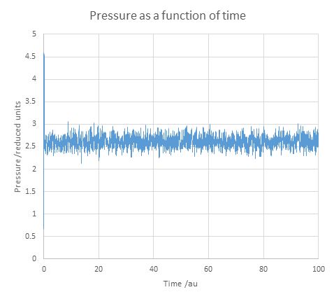
Figure 6. Equilibriation of pressure over time for 0.001 timestep

From Figures 3, 4 and 5 it can be seen that all the calculated parameters reach an equilibrium quickly for the timestep of 0.001, which indicates that it is a particularly precise timestep to use.

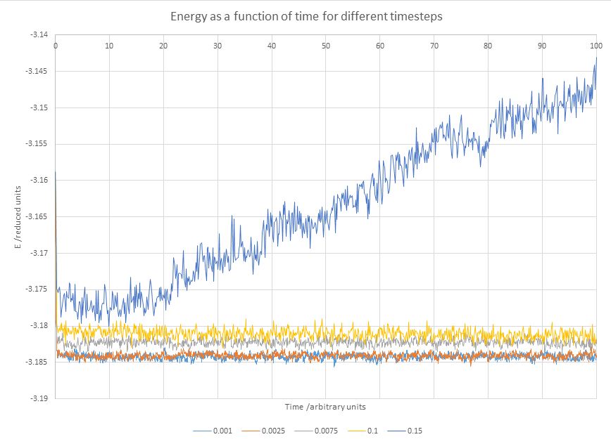
Figure 7. Comparison of equilibriation of energy over time between different timesteps

Figure 8 Average energy for each equilibriated timestep.

In Figure 7 it is visible that all timesteps equal to and lower than 0.01 reach an equilibrium, meaning that they all can be used for simulations to varying degrees of success. The 0.015 timestep fails to reach an equilibrium at all and also provides a visibly different energy than the others, indicating that it cannot be used to simulate the liquids.

From the remaining timestep values the average energies were extracted (Figure 8); it becomes evident that the difference between the 0.001 and 0.0025 timesteps is insignificant, while those for the higher timesteps are further from physical reality. Given the closeness of their results, 0.0025 timestep is a better choice than 0.001, as the same number of steps can cover 2.5 more time with a fixed number of steps simulated. Though not relevant to this particular simulation, this can become useful in situations when the system takes longer to reach an equilibrium, or to save computational resources.

JC: Good choice of timestep, average energy shouldn't depend on the timestep.

Simulations under specific conditions

Setting up the system

We know that: $\frac{1}{2}\sum _i{m}_i{v}_i^2=\frac{3}{2}N{k}_{B}T$

Also at the end of each time step each velocity is multiplied by $\gamma$ to give the desired temperature $\mathfrak{𝔗}$, therefore:

$\frac{1}{2}\sum _i{m}_i(\gamma v_i{)}^2=\frac{3}{2}N{k}_B\mathfrak{𝔗}$

$\frac{{\gamma }^2}{2}\sum _i{m}_i{v}_i^2=\frac{3}{2}N{k}_B\mathfrak{𝔗}$

After dividing by the original equation:

${\gamma }^2=\frac{\mathfrak{𝔗}}{T}$

$\gamma =\sqrt{\frac{\mathfrak{𝔗}}{T}}$

JC: Correct.

In the script there is a line saying:

fix aves all ave/time 100 1000 100000 v_dens v_temp v_press v_dens2 v_temp2 v_press2

The variables starting with v_ show the output values that will be generated at each set interval. The interval at which the output is given is set by the fist number following the ave/time command; in this case it is 100, meaning that the output is generated every 100 timesteps. The second number sets the number of times the input values will be used, in this case, it is 1000 times. The last number (100000) sets the frequency at which the average output values are generated. As the next line of the script is as follows

run 100000

Therefore the average value generated will also be the overall average value, generated from 100000/100=1000 values.

JC: This is a bit unclear.

In order to compare the simulated values to the ideal gas equation, first we must rewrite it in reduced units. The ideal gas law states that

$pV=N{k}_{B}T$

As $p=p^{*}\frac{ϵ}{{\sigma }^3}$ and $T=T^{*}\frac{ϵ}{k_B}$ and $\rho =\frac{{\rho }^{*}}{{\sigma }^3}$, we can substitute these values into the ideal gas equation, which gives the ideal gas equation in reduced units:

${\rho }^{*}=\frac{p^{*}}{T^{*}}$

As we are expressing density as a function of temperature, it is visible that reduced density is inversely proportional to reduced temperature with the gradient of reduced pressure:

${\rho }^{*}=p^{*}\times \frac{1}{T^{*}}$

Analysis of densities

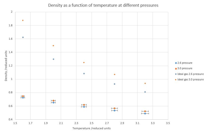
Figure 9. Calculated densities at different temperatures and pressures.

Figure 9 shows that at constant pressure, density is decreasing with temperature. Furthermore, increased pressure increases the density at the same temperature; both of these facts match the physical reality and therefore the simulation has been at least somewhat successful. However, the theoretical density values for an ideal gas are dramatically higher for the same temperature. It is due to the fact that the ideal gas equation completely ignores any intermolecular interactions, including the repulsive ones that dominate at this pressure and cause the atoms to increase their internuclear distances. As the system is warmed up, the discrepancy between both the ideal and non-ideal gas start to disappear, as at higher temperatures densities decrease, the space between atoms increase and real gases start to behave similar to ideal gases.

JC: Good.

Heat capacity

This was the code used to run the heat capacity experiments. New output variables were defined and mentions of pressure were deleted, as it is not necessary to be measured. This code was used to run the simulation at density of 0.2 and temperature of 2.2.

### DEFINE SIMULATION BOX GEOMETRY ###
variable density equal 0.2 
lattice sc ${density}
region box block 0 15 0 15 0 15
create_box 1 box
create_atoms 1 box

### DEFINE PHYSICAL PROPERTIES OF ATOMS ###
mass 1 1.0
pair_style lj/cut/opt 3.0
pair_coeff 1 1 1.0 1.0
neighbor 2.0 bin

### SPECIFY THE REQUIRED THERMODYNAMIC STATE ###
variable T equal 2.2
variable timestep equal 0.0025

### ASSIGN ATOMIC VELOCITIES ###
velocity all create ${T} 12345 dist gaussian rot yes mom yes

### SPECIFY ENSEMBLE ###
timestep ${timestep}
fix nve all nve

### THERMODYNAMIC OUTPUT CONTROL ###
thermo_style custom time etotal temp press
thermo 10

### RECORD TRAJECTORY ###
dump traj all custom 1000 output-1 id x y z

### SPECIFY TIMESTEP ###

### RUN SIMULATION TO MELT CRYSTAL ###
run 10000
reset_timestep 0
unfix nve

### BRING SYSTEM TO REQUIRED STATE ###
variable tdamp equal ${timestep}*100
fix nvt all nvt temp ${T} ${T} ${tdamp}
run 10000
reset_timestep 0
unfix nvt
fix nve all nve

### MEASURE SYSTEM STATE ###
thermo_style custom step etotal temp density atoms
variable dens equal density
variable dens2 equal density*density
variable temper equal temp
variable temper2 equal temp*temp
variable n equal atoms
variable n2 equal atoms*atoms
variable energytotal equal etotal
variable energytotal2 equal etotal*etotal
fix aves all ave/time 100 1000 100000 v_dens v_temper v_dens2 v_temper2 v_energytotal v_energytotal2
run 100000

variable avedens equal f_aves[1]
variable avetemp equal f_aves[2]
variable heatcap equal ${n}*${dens}*(f_aves[6]-f_aves[5]*f_aves[5])/(f_aves[2]*f_aves[2])

print "Averages"
print "--------"
print "Density: ${avedens}"
print "Temperature: ${avetemp}"
print "Heat Capacity: ${heatcap}"

The output of the file can be viewed below:

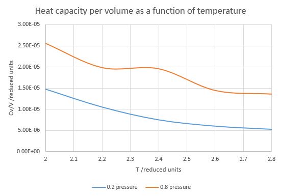
Figure 10. Heat capacity as a function of temperature at p=0.2 and p=0.8

Both pressures show a reduction in heat capacity with increasing temperature (Figure 10). As higher heat capacity correlates with a higher number of rotational, vibrational and other thermally reachable states and more accessible degrees of freedom, it is logical that with increasing temperature the number of states accessible with further increase would drop and therefore the heat capacity would decrease (i.e., more heat energy is converted to kinetic energy in hot molecules than cold molecules). The curve at 0.8 units reduced pressure has a peculiar hump around 2.3-2.4 temperature, indicating that in those particular circumstances there is a higher density of states for some reason that would need further investigation.

It can also be seen that larger pressure applied to a system at a certain temperature would increase the heat capacity over volume. This is due to the fact that now a unit volume contains more molecules and therefore has more accessible states. In other words, the increased pressure increases density and thus the density of states as well.

JC: There is no vibrational or rotational energy in your simulations as you are just simulating spherical particles. Particle density is not necessarily related to density of energy states. A higher pressure and so higher density means more particles per unit volume and so more energy is required per unit volume to raise the temperature.

Radial distribution function

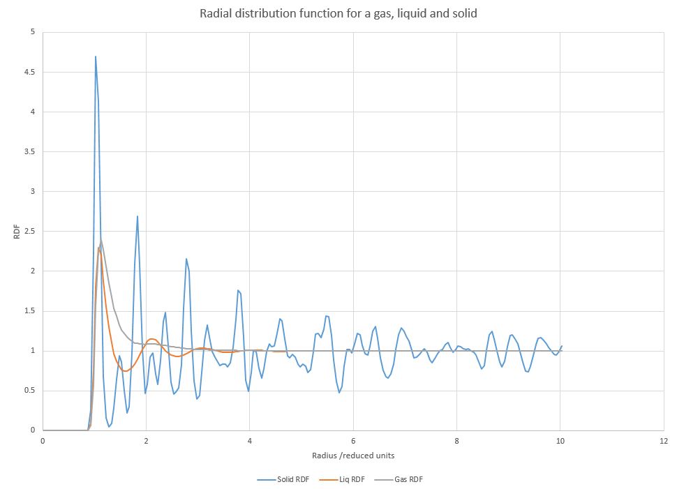
Figure 11. Radial distribution function for a solid, liquid and vapour

Simulations in Figure 11 run at density of 1.15 and temperatures of 0.07, 0.7 and 1.2 to obtain vapour, liquid and solid respectively. The radial distribution functions (RDF) of each phase show some similar features with the the values of 0 up to radii values of around 0.8, followed by one or more peaks and then largely tending to 1. The radial distribution function illustrates the probability of finding at atom at a certain distance from the origin atom. As all atoms repel over short distances, spectra for all three phases show that there there are no other atoms in direct vicinity of the origin atom. Directly outside of this sphere the probability of finding an atom is relatively large, corresponding to the attractive and repulsive parts of Lennard-Jones potential respectively. The function then tends to normalise to 1.

However, there are marked differences in the number of peaks close to atoms in each phase. Gases only get one initial peak, as gas particles interact very weakly and have larger distances between them, therefore they do not have any long-range structure. Liquids show three discernible peaks due to the fact that there exists a short-range structure, as liquid particles are in closer proximity due to existing attractive forces between them. After that, the function tends to 1, indicating a lack of long-range structure. The solids have a large number of peaks, as they exist in crystalline forms and therefore have a large amount of both short-range and long-range structure. Crystals are periodic, therefore as the radius grows, the imaginary sphere crosses either empty space or several atoms in all directions, giving rise to many discernible peaks. Even though the RDF value tends to 1 over time, it can never reach it and shows oscillatory behaviour instead because of the high order of long-range structure present in crystals.

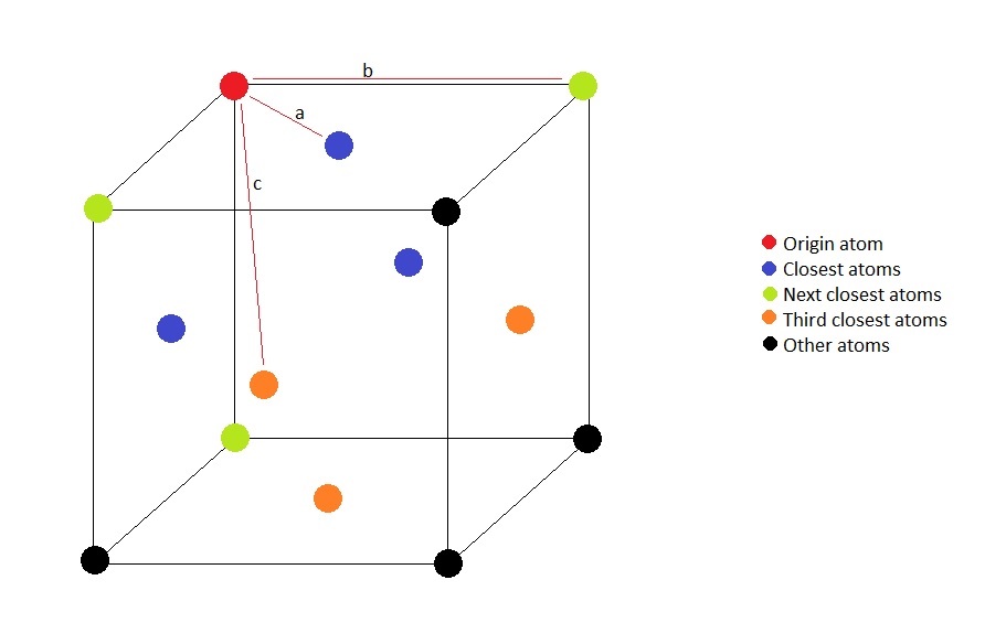
Figure 12. Illustration of the lattice structure.

Illustrated above is the connectivity in the fcc lattice; the red atom is the atom of origin. It is visible that the closest atoms are located on the faces of the cube which intersect at the origin point. The distance a is half of a diagonal of the face of the cube, i.e., it is equal to $\frac{\sqrt{2}}{2}{a}_l$, where $a_l$ is the lattice parameter. The next closest atoms is the corner of the cube, and distance b is therefore equal to the lattice paramter. Third closest atoms can be found on the centres of the faces of the cube that do not contain the origin point. The distance c can be calculated as the hypotenuse of the right triangle one side of which is distance a and the other one is one side of distance b, it is therefore $c=\sqrt{1^2+(\frac{\sqrt{2}}{2}{)}^2}{a}_l=\sqrt{\frac{3}{2}}{a}_l$. The positions of the first three peaks on the RDF rougly correspond to the coefficients of the theoretical distance values by a factor of 1.5, as they are at radii of 1.025, 1.475 and 1.925 respectively.

The area under each peak is proportional to the number of atoms it corresponds to. As the origin atom is in the corner of this cube, it is also simulatanously part of $2^3=8$ cubes, and so are the atoms close to it. There are 3 blue atoms in each of the 8 cubes, but each blue atom is on the face of the cube and is therefore shared between two cubes, so there are $\frac{3\times 8}{2}=12$ blue atoms coordinated with the origin atom.

There are 3 green atoms in each of the 8 cubes in the coordination sphere, however, as each green atom is on the corner of the adjacent cubes, each of them is shared between 4 cubes in the coordination sphere, therefore $\frac{3\times 8}{4}=6$ green atoms coordinate with the origin.

None of the orange atoms are part of another cube in the coordination sphere, therefore there are $3\times 8=24$ orange atoms within distance c of the origin atom.

From the obtained values we can see that the intensity of each peak also mathces what is expected from theory, therefore it can be concluded that the RDF provides useful information about both long-range and short-range structure of solids.

JC: Good idea to express the distances to the first 3 peaks in terms of the lattice parameter - calculate an average lattice parameter from this that you can compare with the value of the initial lattice. The expected number of atoms contributing to each peak are well worked out, but did you check these values with the integral of the RDF, show this graph.

Dynamical properties and diffusion coefficient

Mean square displacement

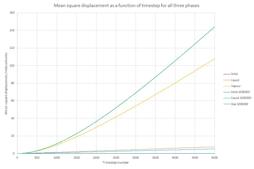
Figure 13. Mean square displacement for a gas, liquid and solid.

In Figure 13, the calculated values are represented with a warm (red-orange-gold) colour scheme, while the given values from 1000000 atoms are shown with a cool (blue-turquoise-green) colour scheme.

The simulated values completely correspond to what is expected from theory: in solid phase the atoms remain almost completely static due to their being in a crystal structure. In both liquid phase and vapour phase the mean square displacement (MSD) increases with time, tending towards a straight line behaviour (pure diffusive behaviour). As liquids have more attractive forces than gases and they are denser, clearly the MSD should be much lower in them than vapour phase; indeed, this behaviour is corroborated by the calculated values.

The provided results of a simulation of 1000000 atoms shows a very similar qualitative behaviour, especially in the solid phase. The provided simulation shows a somewhat lower rate of increase in MSD than the independently run calculation with the opposite being true for the vapour phases. However, it is difficult to speculate about the reasons why this could be the case due to the uncertainty about what conditions were used in the simulations provided.

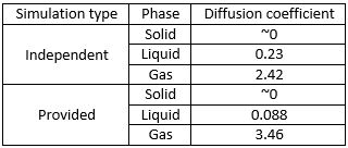
As it is known that $D=\frac{1}{6}\frac{\delta ⟨r^2(t)⟩}{\delta t}$, it can also be seen that the diffusion coefficient is $\frac{1}{6}$ of the gradient at the linear component of the curve. As the graph shows the gradient in the units of the timestep, each gradient has to be divided by the length of the timestep (0.002). The obtained diffusion coefficients are as shown in Figure 14:

Figure 14. Diffusion coefficients as obtained from the gradients of MSD functions

As can be seen, the diffusion coefficient is negligible in solids and about an order of magnitude larger in gases than it is in liquids. A relatively good agreement between the independently simulated values and the values obtained from the provided data can be observed. As diffusion is measured in units of distance squared over time, in this case the units change depending on what the reduced length is equal to as well as the length of one time unit used.

JC: Why does the gas MSD start off as a curved line, what does this represent? Show the lines of best fit on the graphs.

Velocity autocorrection function

The velocity autocorrection function (VACF) for a harmonic oscillator can be solved as follows: It is known that $C(\tau )=\frac{\underset{-\mathrm{\infty }}{\overset{\mathrm{\infty }}{\int }}v(t)v(t+\tau )dt}{\underset{-\mathrm{\infty }}{\overset{\mathrm{\infty }}{\int }}{v}^{2}dt}$

It is also known that harmonic oscillator is described by $x(t)=A\cos (\omega t+\varphi )$, which differentiates into $v(t)=-A\omega \sin (\omega t+\varphi )$

Let us substitute it into the autocorrection formula:

$C(\tau )=\frac{\underset{-\mathrm{\infty }}{\overset{\mathrm{\infty }}{\int }}A\omega \sin (\omega t+\varphi )A\omega \sin (\omega (t+\tau )+\varphi )dt}{\underset{-\mathrm{\infty }}{\overset{\mathrm{\infty }}{\int }}(A\omega \sin (\omega t+\varphi ){)}^{2}dt}$

$A^2$ and ${\omega }^2$ cancel out (constants); $\sin (\omega (t+\tau )+\varphi )$ expanded as per a basic trigonometric identity

$C(\tau )=\frac{\underset{-\mathrm{\infty }}{\overset{\mathrm{\infty }}{\int }}\sin (\omega t+\varphi )(\sin (\omega t+\varphi )\cos (\omega \tau )+(\sin (\omega \tau )\cos (\omega t+\varphi ))dt}{\underset{-\mathrm{\infty }}{\overset{\mathrm{\infty }}{\int }}{\sin }^2(\omega t+\varphi )dt}$

separate and bring out constants:

$C(\tau )=\frac{\cos (\omega \tau )\underset{-\mathrm{\infty }}{\overset{\mathrm{\infty }}{\int }}{\sin }^{}(\omega t+\varphi )dt}{\underset{-\mathrm{\infty }}{\overset{\mathrm{\infty }}{\int }}{\sin }^2(\omega t+\varphi )dt}+\frac{\sin (\omega \tau )\underset{-\mathrm{\infty }}{\overset{\mathrm{\infty }}{\int }}\sin (\omega t+\varphi )\cos (\omega t+\varphi )dt}{\underset{-\mathrm{\infty }}{\overset{\mathrm{\infty }}{\int }}{\sin }^2(\omega t+\varphi )dt}$

In the left hand side summand $\underset{-\mathrm{\infty }}{\overset{\mathrm{\infty }}{\int }}{\sin }^2(\omega t+\varphi )dt$ cancel out; in the right hand side summand the odd function $\sin (\omega t+\varphi )\cos (\omega t+\varphi )$ is integrated over the real number axis, giving 0 as the value of the second summand. Therefore:

$c(\tau )=\cos (\omega \tau )$

JC: Good, clear derivation.

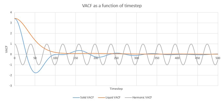
Figure 15. Velocity autocorrection functions for a liquid, a solid and a harmonic oscillator.

As is seen in the Figure 15, both for the liquid and the gas VACF values start high and then with different degrees of oscillatory behaviour approach 0, which means complete lack of correlation. It makes physical sense, as in the beginning the original velocity is the only velocity, but its effect starts to decrease as kinetic energy either is lost to rotational/vibrational energy or is affected by collisions with other particles. Subsequently, the harmonic oscillator correctly predicts oscillations and both liquids and gases tend to change their velocity over time until the original velocity has very little impact on the final velocity. The difference lies in the fact that for solids the oscillation phase lasts much longer, while liquids tend to decorrelate faster. This is due to liquids being in a less structured environment with a larger risk of collision, while for solids in crystalline environments collisions are more limited and they have less kinetic energy, therefore it takes longer to lose the original velocity.

The harmonic VACFs show oscillations, but not the decay to 0 present in the simulated functions. This is due to the fact that harmonic approximation is only valid for atoms in vacuum or very close to the bottom of the Lennard_Jones well and does not take into account the inherent anharmonicity of the system or the possibility of collisions, meaning that the original velocity remains.

Figure 16. Diffusion coefficients as obtained from VACF graphs by trapezoidal method.

From Figure 16 it can be seen that the diffusion coefficients vary widely between the independent simulation and the given data for a million atoms. For solids the trapezoidal method proved especially difficult, as the diffusion coefficient is close to 0 and it does not offer that level of precision. Both precision and accuracy are issues when using the trapezoidal method on VACF graphs, however, when compared to the values obtained by using the gradient (Figure 14), the value for all three easily matched to the same order of magnitude and even better (0.088 obtained for both liquids simulated with 1,000,000 atoms). Therefore it can be concluded the using the trapezoidal method provides a good estimate of what the diffusion coefficient might be.

JC: Again, there is no vibrational or rotational energy in these simulations. Can you be more specific about what the oscillations in the solid and liquid VACFs represent physically?

Conclusion

Molecular dynamics simulations can be used to obtain a large volume of quality data that would otherwise be less accessible due to how even simple models can provide relatively accurate data. They can be used as a tool to investigate new systems with desired properties and supplement purely experimental data collection.