Talk:Mod:fpp1994

Introduction to Molecular Dynamics

File:FrankTASK1.xls

File:FppTASK2.xls

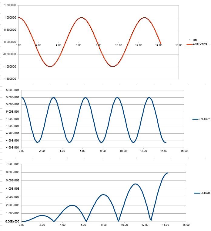
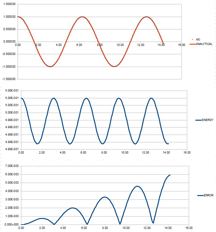
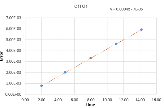
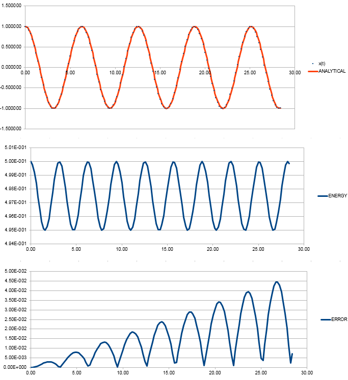
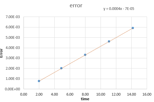
File:FppTASK3.xls Here, it can be seen that when the time-step is 0.2 the total energy fluctuates by 1%. It is important to model the energy of a system you are modelling because in some cases it can be used to calculate thermodynamic quantities as energy is what will dictate how things behave. NJ: It's more important to monitor the conservation of energy, this is an indicator of how well the numerical algorithm is modelling the system. NJ: Why do you think the error accumulates in the way that it does?

---

Task 4

• If $\varphi \left(r\right)=0=4ϵ(\frac{{\sigma }^{12}}{r^{12}}-\frac{{\sigma }^6}{r^6})$

$\frac{{\sigma }^{12}}{r^{12}}=\frac{{\sigma }^6}{r^6}$

${\sigma }^6=r^6$

Thus $\sigma =r_0$ ie $\sigma$ is the distance when the potential is zero

• At this seperation, the force is $\frac{-24ϵ}{r_0}$

$F=\frac{dU}{r}=4ϵ(\frac{-12{\sigma }^{12}}{r^{13}}+\frac{-6{\sigma }^6}{r^7})$ and $\sigma =r=r_0$

$F=24ϵ(\frac{-2}{r_0}+\frac{1}{r_0})=-\frac{24ϵ}{r_0}$

NJ: Be careful with the notation, $F=-\frac{dU}{dr}$, so this is out by a factor of -1.

• The equilibrium seperation, $r=r_{eq}$ occurs at the bottom of the well, so force is at a minimum.

NJ: The potential is at a minimum, so the force is zero.

$F=\frac{dU}{r}=0=4ϵ(\frac{-12{\sigma }^{12}}{r_{eq}^{13}}+\frac{6{\sigma }^6}{r_{eq}^7})$

$\frac{12{\sigma }^{12}}{r_{eq}^{13}}=\frac{6{\sigma }^6}{r_{eq}^7}$

$r_{eq}^6=2{\sigma }^6=2r_0^6$

$r_{eq}=r_0\sqrt[6]{2}=1.122r_0$

• $\varphi \left(r_{eq}\right)=4ϵ(\frac{r_0^{12}}{r_{eq}^{12}}-\frac{r_0^6}{r_{eq}^6})$ and from just above $r_{eq}=r_0\sqrt[6]{2}$

NJ: Good

So $\varphi \left(r_{eq}\right)=4ϵ(\frac{r_0^{12}}{2^6{r}_0^{12}}-\frac{r_0^6}{2r_0^6})=4ϵ(\frac{1}{2^6}-\frac{1}{2})=1.936ϵ$ NJ: You should get a value of $ϵ$ here

---

$\underset{2\sigma }{\overset{\mathrm{\infty }}{\int }}\varphi \left(r\right)\mathrm{d}r=4ϵ{[-\frac{{\sigma }^{12}}{11r^{11}}+\frac{{\sigma }^6}{5r^5}]}_{2\sigma }^{\mathrm{\infty }}$

The expansion of the above bracket is $4ϵ((-\frac{{\sigma }^{12}}{11{\left(\mathrm{\infty }\right)}^{11}}+\frac{{\sigma }^6}{5{\left(\mathrm{\infty }\right)}^5})-(-\frac{{\sigma }^{12}}{11{\left(2\sigma \right)}^{11}}+\frac{{\sigma }^6}{5{\left(2\sigma \right)}^5}))$ but since $\frac{1}{{\mathrm{\infty }}^n}=0$ and $ϵ=\sigma =1$ this becomes $4(\frac{1}{11{\left(2\right)}^{11}}-\frac{1}{5{\left(2\right)}^5})=-0.0248$

Using the same expansion, but $2.5\sigma$ and $3\sigma$ as the lower limits gives $-0.00818$ and $-0.00329$ respectively.

NJ: Good

---

Task 5:

The density of water is $$\begin{gathered} 1000{\mathrm{k}\mathrm{g} \\ \mathrm{m}}^{-3} \end{gathered}$$ and so $1\mathrm{m}\mathrm{L}$ would weigh $1\mathrm{g}$. The molecular mass of water is $18.0{\mathrm{g}\mathrm{m}\mathrm{o}\mathrm{l}}^{-1}$ and so the amount of molecules in $1\mathrm{m}\mathrm{L}$ of water is $1/18\times N_A=3.35\times 10^{22}$. Therefore $10000$ molecules would occupy $\frac{10000}{3.35\times 10^{22}}=2.99\times 10^{-18}\mathrm{m}\mathrm{L}$.

NJ: Good

---

Task 6

Consider an atom at position $(0.5,0.5,0.5)$ in a cubic simulation box which runs from $(0,0,0)$ to $(1,1,1)$. In a single timestep, it moves along the vector $(0.7,0.6,0.2)$. At what point does it end up, after the periodic boundary conditions have been applied?. It would be at $(0.2,0.1,0.7)$

---

Task 7

• $r^{*}=\frac{r}{\sigma }$ therefore $r^{*}\sigma =r=0.34\times 10^{-9}\times 3.2=1.08\times 10^{-9}\mathrm{m}$

NJ: 1.088nm

• If $\frac{ϵ}{k_B}=120\mathrm{K}$ then since $k_B=1.38\times 10^{-23}$ the well depth in $\mathrm{k}\mathrm{J}\mathrm{m}\mathrm{o}{\mathrm{l}}^{\mathrm{-}\mathrm{1}}$ is $ϵ=120\times 1.38\times 10^{-23}\times 1000=1.66\times 10^{-18}\mathrm{k}\mathrm{J}\mathrm{m}\mathrm{o}{\mathrm{l}}^{\mathrm{-}\mathrm{1}}$

NJ: This is just in kJ, not kJ per mole.

• temperature $T^{*}=\frac{k_{B}T}{ϵ}$ therefore $T=\frac{T^{*}ϵ}{k_B}=1.5\times 120=180\mathrm{K}$

Equilibration

Task 1 Giving atoms random starting positions in simulations can cause problems because if there are two atoms that are placed too close together (ie if they are within $r_0$ of each other) then their potential energies - and thus initial accelerations and velocities -will be extremely high and they will move through the sample with an unrealistically high speed and this will also disrupt other atoms.

NJ: Good. Can you say a bit more about this? Why won't this energy just be dissipated through the system?

---

Task 2

If each the spacing lattice point is 1.07722 and the lattice is three dimensional then the number density of lattice point is given by $\frac{1}{spacing}=\frac{1}{1.07722^3}=0.8$

If a face-centred cubic lattice has a number density of 1.2 then because it has four atoms per cell its volume can be given by $V=\frac{number}{density}=\frac{4}{1.2}$ and so the side length is just the cube root of this and so $l=\sqrt[3]{\frac{4}{1.2}}=1.49$

Task 3

In the same lattice if the command "create_atoms" was used, 4000 atoms would be created as there are 4 atoms per unit cell.

NJ: Good. Nicely explained.

---

Task 4

mass 1 1.0
pair_style lj/cut 3.0
pair_coeff * * 1.0 1.0

The first command sets the relative mass of Atom 1 as 1. NJ: Good effort, but it's the mass of all atoms of type one, not just the mass of the first atom. In the second command "pair_style" is used to describe interactions between two particles and the "lj/cut" part tells LAMMPS that this interaction follows the Lennard-Jones potential and nothing more and that it cuts of when $r=3$.

"pair_coeff" tells LAMMPS what coefficients to use in the style defined above. In this case it is the Lennard-Jones potential, and so it is telling LAMMPS to set $ϵ$ and $\sigma$ as 1. NJ: Good

---

Task 5 Specifying velocity and position as starting conditions means the Velocity Verlet Algorithm should be used.

---

Task 6

Specifying variables rather than numerical values useful is because you may need to use that value at various points throughout the script. Using numerical values all over the script would become particularly annoying if you were running lots of simulations with the same variable multiple times as you would have to look through the whole script to find each value but with the dollar command you can just change it once. NJ: This section makes sure that the same length of time is simulated no matter what timestep is chosen.

Task 7

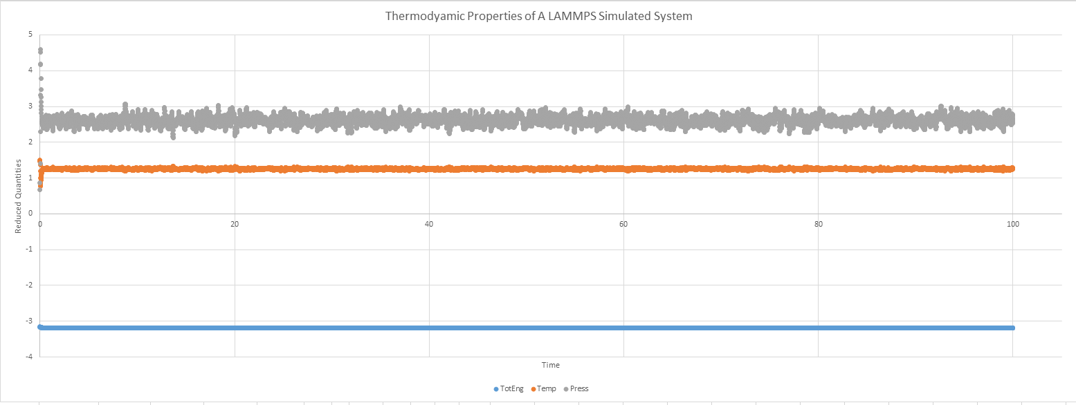
The system reaches equilibrium after a time of about 0.5

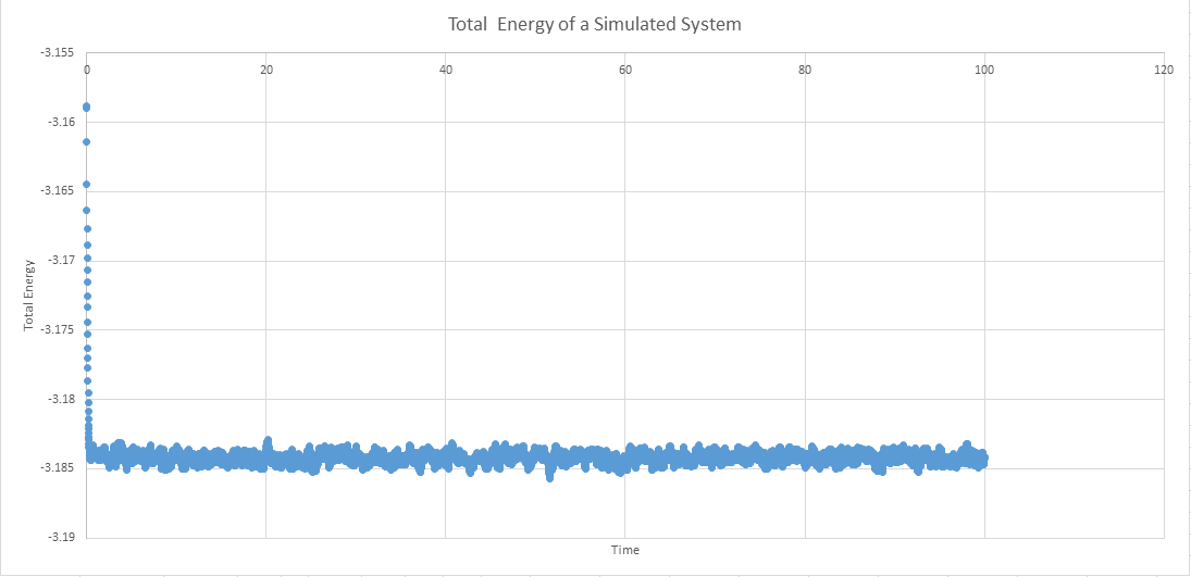
5 simulations were run with timestops of 0.001, 0.01, 0.0025, 0.0075, 0.015. The worst choice is the one with the highest timestop, 0.015 because ideally a balance between resolution and the amount of time the system can be monitored is preferred but all of the timestops show the eventual equilibrium and so there is little benefit to a large value as instead it does not show the fact that equilibrium had to be reached.

NJ: There should be a plot of energy as a function of time for all five timesteps, on the same axes. You should find that 0.015 does not reach equilibrium. What timestep did you choose for the rest of your simulations?

Running simulations under specific conditions

Task 1

10 phase points (two pressures and 5 temperatures) were selected, $T^{*}=1.6,1.8,2.0,2.2,2.4$ and $p^{*}=2.4,2.8$ and the timestep was 0.001

Task 2

$\frac{1}{2}\sum _i{m}_i{v}_i^2=\frac{3}{2}N{k}_{B}T$

$$\begin{gathered} \frac{1}{2}\sum _i{m}_i{\left(\gamma v_i\right)}^2={\gamma }^2\frac{1}{2}\sum _i{m}_i{v}_i^2 \\ =\frac{3}{2}N{k}_B\mathfrak{𝔗} \end{gathered}$$

$\frac{\frac{1}{2}\sum _i{m}_i{v}_i^2}{T}=\frac{3}{2}N{k}_B$ therefore ${\gamma }^2\frac{1}{2}\sum _i{m}_i{v}_i^2=\frac{\frac{1}{2}\sum _i{m}_i{v}_i^2}{T}\mathfrak{𝔗}$

Cancel $\frac{1}{2}\sum _i{m}_i{v}_i^2$ to give ${\gamma }^2=\frac{\mathfrak{𝔗}}{T}$

Task 3

From the script

 fix aves all ave/time 100 1000 100000 v_dens v_temp v_press v_dens2 v_temp2 v_press2 

From the LAMMPS manual

 fix ID group-ID ave/time Nevery Nrepeat Nfreq value1 value2 ... keyword args ...

The numbers 100, 1000 and 100000 correspond to Nevery, Nrepeat and Nfreq respectively. These commands tell LAMMPS on which timesteps to calculate the averages of the properties that follow. Nrepeat tells LAMMPS how many averages to calculate, starting from the value given by Nfreq and working back in multiples of Nevery. In this case 1000 averages are taken in total, once every 100 timesteps up to 100000 which is as far as the script will run.

Task 4

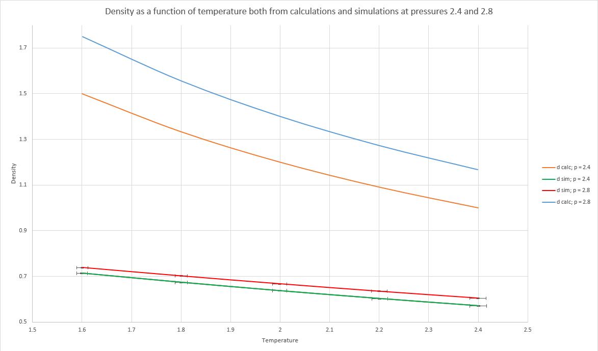
The bottom two lines are the density as a function of temperature as calculated by LAMMPS whereas the top lines are calculated using the ideal gas law using the equation derived below where pressure was 2.4 and 2.8 and the temperature was the LAMMPS average. The simulated density is much lower than the one predicted by the gas law because the gas is not ideal as there are repulsive and attractive terms in the Lennard-Jones potential and ideal gases have no interaction between the particles. NJ: Good, but why do you always find a lower density in the simulations?And as the pressure increases the gap between the simulated and calculated densities increases too because at higher pressures there are more interaction between the particles and so the ideal gas approximation gets worse. NJ: Good. What about the trend with temperature?

$PV=N{k}_{B}T$

$P=\frac{N}{V}{k}_{B}T$ and $\rho =\frac{N}{V}$

so $P=\rho k_{B}T$ but on LAMMPS in lj style, $ϵ,\sigma$ and $k_B$ are all equal to 1

so $\frac{P}{T}=\rho$

Calculating heat capacities using statistical physics

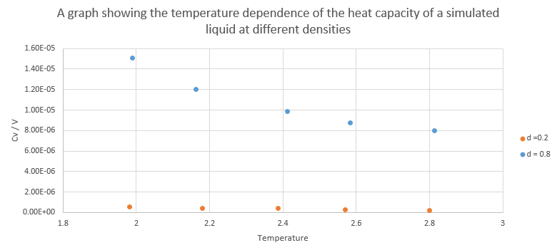
The script used to calculate the heat capacities is below

### DEFINE SIMULATION BOX GEOMETRY ###
variable density equal  0.2
lattice sc ${density}
region box block 0 15 0 15 0 15
create_box 1 box
create_atoms 1 box
variable atoms equal 15*15*15*${density}

### DEFINE PHYSICAL PROPERTIES OF ATOMS ###
mass 1 1.0
pair_style lj/cut/opt 3.0
pair_coeff 1 1 1.0 1.0
neighbor 2.0 bin

### SPECIFY THE REQUIRED THERMODYNAMIC STATE ###
variable T equal 2.0

variable timestep equal 0.001

### ASSIGN ATOMIC VELOCITIES ###
velocity all create ${T} 12345 dist gaussian rot yes mom yes

### SPECIFY ENSEMBLE ###
timestep ${timestep}
fix nve all nve

### THERMODYNAMIC OUTPUT CONTROL ###
thermo_style custom time etotal temp press
thermo 10

### RECORD TRAJECTORY ###
dump traj all custom 1000 output-1 id x y z

### SPECIFY TIMESTEP ###

### RUN SIMULATION TO MELT CRYSTAL ###
run 10000
unfix nve
reset_timestep 0

### BRING SYSTEM TO REQUIRED STATE ###
variable tdamp equal ${timestep}*100
variable pdamp equal ${timestep}*1000
fix nvt all nvt temp ${T} ${T} ${tdamp} 
run 10000
reset_timestep 0
unfix nvt
fix nve all nve

### MEASURE SYSTEM STATE ###
thermo_style custom step etotal temp press density
variable dens equal density
variable dens2 equal density*density
variable temp equal temp
variable temp2 equal temp*temp
variable press equal press
variable press2 equal press*press
variable etotal equal etotal
variable etotal2 equal etotal*etotal
fix aves all ave/time 100 1000 100000 v_dens v_temp v_press v_dens2 v_temp2 v_press2 v_etotal v_etotal2
run 100000

variable avedens equal f_aves[1]
variable avetemp equal f_aves[2]
variable avepress equal f_aves[3]
variable aveetotal equal f_aves[7]
variable aveetotal2 equal f_aves[8]
variable errdens equal sqrt(f_aves[4]-f_aves[1]*f_aves[1])
variable errtemp equal sqrt(f_aves[5]-f_aves[2]*f_aves[2])
variable errpress equal sqrt(f_aves[6]-f_aves[3]*f_aves[3])
variable heatcap equal ${atoms}*${atoms}*((f_aves[8]-f_aves[7]*f_aves[7])/(f_aves[2]*f_aves[2]))

print "Averages"
print "--------"
print "Density: ${avedens}"
print "Stderr: ${errdens}"
print "Temperature: ${avetemp}"
print "Stderr: ${errtemp}"
print "Pressure: ${avepress}"
print "Stderr: ${errpress}"
print "Heat capacity: ${heatcap}"

NJ: The number of atoms isn't given by 15*15*15*density, it's just 15^3. You've got the correct trend, but the absolute values are a bit out. Can you explain how this varies with density and temperature?

Structural properties and the radial distribution function

NJ: Nice plot The solid is face-centred cubic and so when a reference atom is defined, there are 3 different distances that the other atoms in the unit cell can be away from each other. NJ: Only three?If the reference atom is in the middle of the top face of the cube, out of the first three peaks, the smallest (and second) peak will be from the atom in the middle of the opposite face of the cell because there are 4 atoms that fit this description, also the RDF has also been normalised and this is a relationship between two of the same lattice points and so it makes sense that the density at this point would be 1. The first peak will be the atoms on the corners of the same face as the reference atom and the atoms that are in the middle of the cell’s remaining faces as they are all the same distance from the reference atom; this is because the distance as you go to an edge and go down is the same as if you go to the edge and go across since the cell is a cube, also there are 12 such atoms and this is the tallest peak. The third peak arises from the atoms that are on the corners of the opposite face of which there are 8. The numbers quoted all arise from considering the actual lattice rather than the cell and also compare well with the relative heights of the peaks.

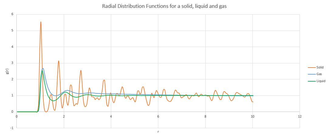
NJ: I think there's a little bit of confusion here - whichever reference atom you pick, the lattice looks the same in all directions. The RDF is also averaged over all atoms. I wanted you to work out the interatomic distances in terms of the lattice constant for the first three peaks, and calculate the spacing using your graph, rather than reading from the log file. You also should have used the integrated g(r) data to calculate the coordination number for each of the first three peaks.

The RDF for liquids and gases look quite similar to each other but different to that of the solid as they are much less ordered. In both cases, the first peak is quite large before the curve quickly levels out at 1. The RDF measures the amount of atoms in a shell of radius, r, around the reference atom and so when the shell is small the concentration of nearby atoms is high and they resemble clusters. However, as the shell gets bigger it starts to become more diffuse and eventually reaches a point where the concentration of atoms in the shell cannot be distinguished from the density of the system as a whole.

NJ: What density did you use for the gas? As you say, it looks very similar to the liquid. I suspect this is a bit too dense, and is in the liquid/gas coexistence region. Why does the solid RDF have so many more defined peaks?

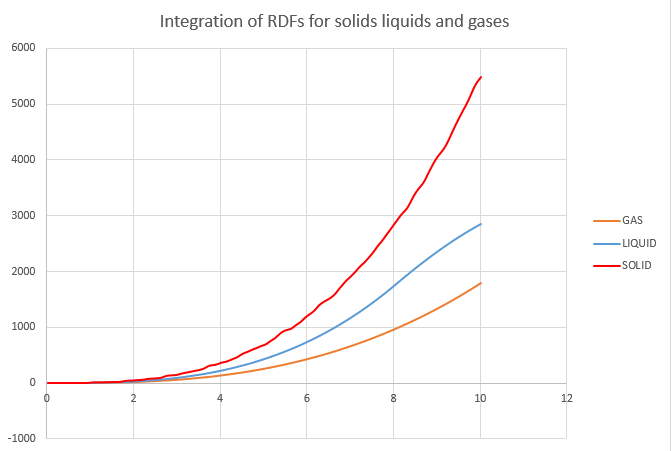
By eye, the liquid and gas RDFs would seem to suggest that the gas is ever so slightly denser than the liquid, however, the functions are normalised and the actual density of gases is much lower and so there are far fewer atoms than in the liquid, as can be seen in the plots of their integrations.

From the log file, the lattice spacing of the solid is

Lattice spacing in x,y,z = 1.45447 1.45447 1.45447

Dynamical properties and the diffusion coefficient

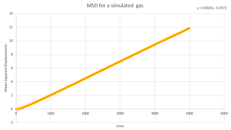
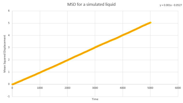
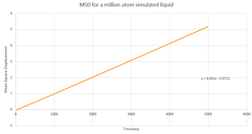
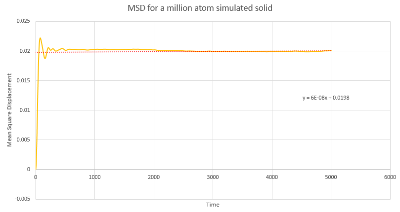
NJ: Be careful, these values are all in reduced units.

$D=\frac{1}{6}\times 0.0025=4.17\times 10^{-4}{m}^{2}timestep{}^{-}1$

$D=\frac{1}{6}\times 0.001=1.66\times 10^{-4}{m}^{2}timeste{p}^{-1}$

$D=\frac{1}{6}\times 0.0025=1.33\times 10^{-6}{m}^{2}timeste{p}^{-1}$ NJ: Do you think this is a realistic MSD for a solid? Why does it look so different to the result for the 1 million atoms simulation?

$D=\frac{1}{6}\times 0.0305=0.00508m^{2}timeste{p}^{-1}$ NJ: You should only fit the straight line to the linear region. Why do you think this graph is curved?

$D=\frac{1}{6}\times 0.001=1.66\times 10^{-4}{m}^{2}timeste{p}^{-1}$

$D=\frac{1}{6}\times 6\times 10^{-8}=1\times 10^{-8}{m}^{2}timeste{p}^{-1}$

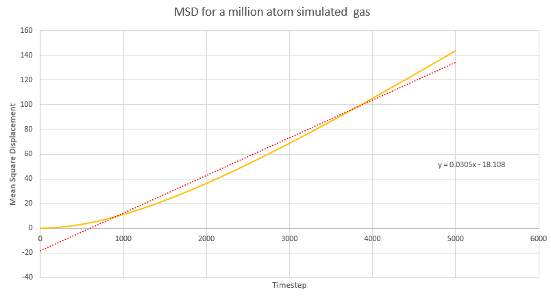
NJ: How do the values of D compare across phases? Does using 1 million atoms make a difference?

$x\left(t\right)=A\cos (\omega t+\varphi )$

$x^{\prime }\left(t\right)=v(t)=-A\omega \sin (\omega t+\varphi )$

$v^2(t)=A^2\omega {\sin }^2(\omega t+\varphi )$

$v(t+\tau )=-A\omega \sin (\omega t+\omega \tau +\varphi )$ define: $\alpha =\omega t+\varphi$

$v(t+\tau )=-A\omega \sin (\alpha +\omega \tau )=-A\omega \sin \left(\alpha \right)\cos \left(\omega \tau \right)\sin \left(\omega \tau \right)\cos \left(\alpha \right)$

$C\left(\tau \right)=\frac{\underset{-\mathrm{\infty }}{\overset{\mathrm{\infty }}{\int }}v\left(t\right)v(t+\tau )\mathrm{d}t}{\underset{-\mathrm{\infty }}{\overset{\mathrm{\infty }}{\int }}{v}^2\left(t\right)\mathrm{d}t}=\frac{\underset{-\mathrm{\infty }}{\overset{\mathrm{\infty }}{\int }}{A}^2{\omega }^2{\sin }^2\left(\alpha \right)\cos \left(\omega \tau \right)+\sin \left(\omega \tau \right)\cos \left(\alpha \right)\mathrm{d}\alpha }{\underset{-\mathrm{\infty }}{\overset{\mathrm{\infty }}{\int }}{A}^2\omega {\sin }^2\left(\alpha \right)\mathrm{d}\alpha }$ NJ: This is the right start.