Talk:Mod:fiercemonkey

All results in this report, unless otherwise stated, are in reduced units. All values were calculated and presented with constants set to 1.

LAMMPS input commands, data extraction and presentation were done using Python and MatPlotLib. The codes for these scripts can be found here.

Section 1: Introduction Molecular Dynamics Simulation

Verlet Algorithm

Harmonic Oscillator model

The analytical solution to the position of x is $A\cos (\omega t)$ and is compared to the result from the velocity Verlet algorithm, which takes snapshots of the oscillator to calculate the elastic force, $F=-kx$ and iterate onto the next snapshot. Both position and potential energy agree with the harmonic oscillator model, which is not surprising as the force in the Verlet algorithm uses Hooke's law.

NJ: Not necessarily. You can use the Verlet algorithm with any potential function that you like, it's just that this is the form you need for a harmonic oscillator.

From the last plot illustrating the absolute error over time, it is clear that each iteration of the velocity Verlet algorithm carries errors from its previous oscillations. The maxima in each oscillation is found and tabulated below.

Time	Maximum % Error in Energy
2.0	0.08%
4.9	0.20%
8.0	0.33%
11.1	0.46%
14.2	0.59%

The linear plot shows the absolute error increases over time in a $0.0004t|\sin (\omega t)|$ fashion. Note that at energy minima, the error accumulates over each successive cycle. The velocity Verlet algorithm does not reach the exact equilibrium point, and always calculates a non-zero energy, which accumulates over time to give this pattern.

NJ: But the energy of a moving harmonic oscillator isn't zero...

Effect of Timestep Used

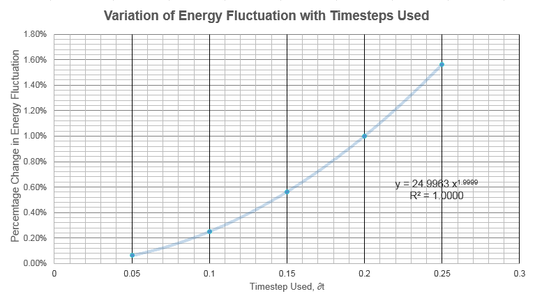
Smaller timesteps resulted in smaller errors. The largest timestep that produced a less-than-1% error in total energy is $\partial t=0.20$. The second law of thermodynamics dictates that the total energy in any system must be constant, and therefore the system with the lowest variation in total system energy must be the most accurate picture of the ensemble.

NJ: Good, but it's the law of conservation of energy that means the energy should be constant, not the second law. The second law says that the total entropy of the universe must increase.

Atomic Forces

Lennard-Jones Potential

The Potential Energy function is zero when:

$\begin{array}{rl}\varphi (r_0)=4ϵ[{\left(\frac{\sigma }{r_0}\right)}^{12}-{\left(\frac{\sigma }{r_0}\right)}^6]& =0\\ {\left(\frac{\sigma }{r_0}\right)}^{12}-{\left(\frac{\sigma }{r_0}\right)}^6& =0\\ {\left(\frac{\sigma }{r_0}\right)}^6& =0\\ r_0& =\sigma \end{array}$

The minima in the Potential Energy function occurs when:

$\begin{array}{rl}{\varphi }^{\prime }(r_e)=4ϵ(-\frac{12{\sigma }^{12}}{r_e^{13}}+\frac{6{\sigma }^6}{r_e^7})& =0\\ (-\frac{12{\sigma }^{12}}{r_e^{13}}+\frac{6{\sigma }^6}{r_e^7})& =0\\ \frac{12{\sigma }^{12}}{r_e^{13}}& =\frac{6{\sigma }^6}{r_e^7}\\ {\left(\frac{\sigma }{r_e}\right)}^6& =2\\ r_e& =2^{\frac{1}{6}}\sigma \end{array}$

NJ: What about the force?

Substituting the equilibrium bond length, we obtain the value of the minimum potential energy:

$\begin{array}{rl}\varphi (r_e)& =4ϵ[{\left(\frac{\sigma }{r_e}\right)}^{12}-{\left(\frac{\sigma }{r_e}\right)}^6]\\ & =4ϵ[\frac{{\sigma }^{12}}{4{\sigma }^{12}}-\frac{{\sigma }^6}{5{\sigma }^5}]\\ & =-ϵ\end{array}$

The integrals can be generalised in the following form:

$\begin{array}{rl}\underset{a\sigma }{\overset{\mathrm{\infty }}{\int }}\varphi (r)\mathrm{d}r& =4ϵ\underset{a\sigma }{\overset{\mathrm{\infty }}{\int }}[{\left(\frac{\sigma }{r}\right)}^{12}-{\left(\frac{\sigma }{r}\right)}^6]\mathrm{d}r\\ & =4ϵ{[-\frac{{\sigma }^{12}}{11r^{11}}+\frac{{\sigma }^6}{5r^5}]}_{a\sigma }^{\mathrm{\infty }}\\ & =\left[0\right]-\left[4ϵ(\frac{-\sigma }{11a^{11}}+\frac{\sigma }{5a^5})\right]\\ & =\frac{4}{11a^{11}}-\frac{4}{5a^5}\text{when }\sigma =ϵ=1.\end{array}$

Substituting different values of $a$,

$\begin{array}{rl}\underset{2\sigma }{\overset{\mathrm{\infty }}{\int }}\varphi (r)\mathrm{d}r& =-0.024822\\ \underset{2.5\sigma }{\overset{\mathrm{\infty }}{\int }}\varphi (r)\mathrm{d}r& =-0.022227\\ \underset{3\sigma }{\overset{\mathrm{\infty }}{\int }}\varphi (r)\mathrm{d}r& =-0.003290\end{array}$

Periodic Boundary Conditions

At stnadard conditions, the density of water is $1{\text{ g mL}}^{-1}$. The mass of 1mL water is therefore $1\text{ g}$. There are $\frac{1\text{ g}\times N_A{\text{ mol}}^{-1}}{M_r{\text{ g mol}}^{-1}}=\frac{N_A}{18.015}=3.3327\times 10^{22}$ molecules in 1mL water.

The mass of 10000 water molecules is $M_r\times \frac{10000}{N_A}=3.00\times 10^{-20}\text{ g}$. At standard conditions, this mass of water occupies $3.00\times 10^{-20}\text{ mL}$ of volume.

NJ: The volume should be of order $10^{-19}$, but good otherwise. Nicely presented.

The position of the moving atom is:

$\begin{array}{rl}x(t+\delta t)=x(t)+v\delta t& =\left(\begin{array}{c}0.5\\ 0.5\\ 0.5\end{array}\right)+\left(\begin{array}{c}0.7\\ 0.6\\ 0.2\end{array}\right)\\ & =\left(\begin{array}{c}1.2\\ 1.1\\ 0.7\end{array}\right)\\ & \equiv \left(\begin{array}{c}1.2\\ 1.1\\ 0.7\end{array}\right)-\left(\begin{array}{c}1\\ 1\\ 0\end{array}\right)\\ & =\left(\begin{array}{c}0.2\\ 0.1\\ 0.2\end{array}\right)\text{after applying the periodic boundary condition.}\end{array}$

NJ: Not (0.2,0.1,0.7)?

Reduced Units

The Lennard-Jones cutoff is:

$r=r^{*}\sigma =3.2\times 0.34\text{nm}=1.088\text{nm}$

From above derivations, $\varphi (r_e)=-ϵ$ at equilibrium bond length in reduced units, therefore $E_{\text{well depth}}^{*}=1$:

$\begin{array}{rl}{E}_{\text{well depth}}=ϵE_{\text{well depth}}^{*}& =E_{\text{well depth}}^{*}\times \left(\frac{ϵ}{k_B}\right)\times k_B\\ & =1\times 120\times k_B{\text{ J K}}^{-1}\\ & =1\times 0.12\times R{\text{ kJ K}}^{-1}{\text{mol}}^{-1}\\ E_{\text{well depth}}& =0.9977{\text{ kJ K}}^{-1}{\text{mol}}^{-1}\end{array}$

The temperature on the Kelvin scale is:

$T=T^{*}\times \left(\frac{ϵ}{k_B}\right)=1.5\times 120=180\text{ K}$

Section 2: Equilibration

Creating the Simulation Box

Starting Positions

Randomnised starting positions may lead to molecules that are too close together, invoking the $r^{-12}$ repulsive interaction in the Lennard-Jones potential, leading to a high-energy system with erratic and unrealistic behavior.

NJ: Good.

On the other hand, some molecules may be too apart and only very weakly attracted to each other, giving a static picture of the system. The randomnised starting position does not include considerations regarding total system energies. We can argue that energy is more important in the respect that we want to simulate an ensemble with realistic conditions.

NJ: This is true, but the system would probably tend quite quickly to equilibrium. The large repulsive forces that you get when atoms overlap, however, are harder to deal with (you need a shorter timestep).

Unit Cell Length

For a simple cubic lattice, there are 4 atoms per unit cell. A number density of 0.8 corresponds to a unit cell length of 1.07722:

$\begin{array}{rl}\text{Number Density}=\frac{n_{\text{cell}}}{V_{\text{cell}}}& =\frac{1}{l^3}\\ 0.8& =\frac{1}{l^3}\\ l& =1.07722\end{array}$

Face-centred cubic cells have 4 atoms per unit cell. From the same formula, a face-centred cell with a number density of 1.2 has the side length of 1.49380.

$\begin{array}{rl}\text{Number Density}=1.2& =\frac{4}{l^3}\\ l& =1.49380\end{array}$

Defining the Lattice

The box is defined to be $10\times 10\times 10=1000$ unit cells, each unit cell containing 4 atoms. The total number of atoms created is $1000\times 4=4000$.

Setting the Properties of Atoms

Given that we are specifying both position and velocity, the integration algorithm used is velocity Verlet.

mass 1 1.0
pair_style lj/cut 3.0
pair_coeff * * 1.0 1.0

The mass of atom 1 is set to 1.0. Since all atoms are identical, this value does not really affect the simulation.

NJ: The mass is part of the conversion factor between reduced time and real time. It would be better to say that since the atoms are identical, they can be taken to have a reduced mass of 1.

pair_style sets the energy interactions between each pair of atoms. The style chosen is Lennard-Jones potential with a cut-off distance. In this case, any interaction between atoms further away than $3.0\sigma$ will not be calculated. pair_coeff sets Lennard-Jones constants globally using the * * command. The 1.0 1.0 refers to Lennard-Jones coefficients $ϵ$ and $\sigma$, respectively.

The integration algorithm used is velocity Verlet.

Running the Simulation

The duration of the simulation is set to a constant, 100 time units. By defining timestep to a variable, the program automatically calculates the number of timesteps required to reach that duration (in the code "variable n_steps equal floor(100/${timestep})"). If this was not done, then the number in "run ${n_steps}" must be calculated and altered each time when the timestep increment is changed.

NJ: Well spotted, and well explained.

Checking Equilibration

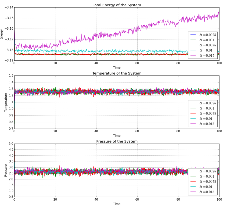
After roughly 0.5 units of time and 500 timesteps, the system reached an equilibrium state. The total energy, temperature and pressure of the system approached a constant value.

The total energy of the 0.015 timestep system keeps increasing, which is clearly impossible since this is an isolated system and the total energy must be conserved. The rest of the systems all reached equilibrium states after roughly the same number of timesteps. The 0.001 timestep system would be the most practical to use, since this requires the least number of steps for the same duration of simulation, and this simulated a good and realistic equilibrium state.

NJ: 0.001 is the smallest timestep, so it would require the largest number of steps.

NJ: I'm assuming you meant 0.01, which is a bit big. We don't really want the average energy to depend on the choice of timestep - the two smallest timesteps, 0.001 and 0.0025 should give approximately the same results. 0.0025 is then the best choice because we get more time out of the simulation for the same number of steps.

Section 3: Running Simulations under Specific Conditions

Temperature and Pressure Control

The tempratures and pressures chosen were $1.0,1.5,2.0,2.5,3.0,3.5,4.0$ and $2.5,4.0$, respectively.

Below is an example input script.

### DEFINE SIMULATION BOX GEOMETRY ###
lattice sc 0.8
region box block 0 15 0 15 0 15
create_box 1 box
create_atoms 1 box

### DEFINE PHYSICAL PROPERTIES OF ATOMS ###
mass 1 1.0
pair_style lj/cut/opt 3.0
pair_coeff 1 1 1.0 1.0
neighbor 2.0 bin

### SPECIFY THE REQUIRED THERMODYNAMIC STATE ###
variable T equal 2
variable p equal 2.5
variable timestep equal 0.0025 

### ASSIGN ATOMIC VELOCITIES ###
 velocity all create ${T} 12345 dist gaussian rot yes mom yes
 
 ### SPECIFY ENSEMBLE ###
 timestep ${timestep}
 fix nve all nve
 
 ### THERMODYNAMIC OUTPUT CONTROL ###
 thermo_style custom time etotal temp press
 thermo 10
 
 ### RECORD TRAJECTORY ###
 dump traj all custom 1000 output-1 id x y z
 
 ### SPECIFY TIMESTEP ###
 
 ### RUN SIMULATION TO MELT CRYSTAL ###
 run 10000
 unfix nve
 reset_timestep 0
 
 ### BRING SYSTEM TO REQUIRED STATE ###
 variable tdamp equal ${timestep}*100
 variable pdamp equal ${timestep}*1000
 fix npt all npt temp ${T} ${T} ${tdamp} iso ${p} ${p} ${pdamp}
 run 10000
 reset_timestep 0
 
 ### MEASURE SYSTEM STATE ###
 thermo_style custom step etotal temp press density
 variable dens equal density
 variable dens2 equal density*density
 variable temp equal temp
 variable temp2 equal temp*temp
 variable press equal press
 variable press2 equal press*press
 fix aves all ave/time 100 1000 100000 v_dens v_temp v_press v_dens2 v_temp2 v_press2
 run 100000
 
 variable avedens equal f_aves[1]
 variable avetemp equal f_aves[2]
 variable avepress equal f_aves[3]
 variable errdens equal sqrt(f_aves[4]-f_aves[1]*f_aves[1])
 variable errtemp equal sqrt(f_aves[5]-f_aves[2]*f_aves[2])
 variable errpress equal sqrt(f_aves[6]-f_aves[3]*f_aves[3])
 
 print "Averages"
 print "--------"
 print "Density: ${avedens}"
 print "Stderr: ${errdens}"
 print "Temperature: ${avetemp}"
 print "Stderr: ${errtemp}"
 print "Pressure: ${avepress}"
 print "Stderr: ${errpress}"

Thermostats and Barostats

Dividing the second equation by the first,

$\begin{array}{rl}\frac{1}{2}\sum _i{m}_i{v}_i^2& =\frac{3}{2}N{k}_{B}T\text{(1)}\\ \frac{1}{2}\sum _i{m}_i{\left(\gamma v_i\right)}^2& =\frac{3}{2}N{k}_B\mathfrak{𝔗}\text{(2)}\\ \frac{\sum _i{m}_i{\gamma }^2{v}_i^2}{\sum _i{m}_i{v}_i^2}& =\frac{\mathfrak{𝔗}}{T}\text{(2)}÷\text{(1)}\\ \gamma & =\sqrt{\frac{\mathfrak{𝔗}}{T}}\end{array}$

Examining the Input Script

fix aves all ave/time 100 1000 100000 v_dens v_temp v_press v_dens2 v_temp2 v_press2

The three numbers 100, 1000, 100000 tells LAMMPS how to sample data to calcualte the averages. Every 100 timesteps, thermodynamics data is saved. This saving action is repeated 1,000 times in the whole of simulation. Every 100,000 steps, an average value of thermodynamics data is calculated and stored.

A total of 100,000 steps is run in this simulation. So one average is calculated, and the average is calculated from 1,000 data points.

The total time simulated is $T^{*}=100,000\text{ steps}\times 0.0025\text{ time per step}=250$.

Plotting the Equations of State

LAMMPS-simulated number density is lower than that predicted by the ideal gas law. At low temperatures, the disagreement becomes greater and the ideal gas law suggests infinite density at absolute zero. At this range of temperature, reduced kinetic energy means that potential energy has a proportionally bigger contribution towards the total system energy. The ideal gas law assumes no potential energy and inter-atom interactions, in contrast with the 12-6 Lennard-Jones potential, which has a sharp repulsive component and prevents obtaining unrealistically high densities. The Lennard-Jones potential models atoms very closely as hard spheres, whereas the particles are only points with infinite packing in the ideal gas law.

At high pressures, the number density increases over all temperatures. This is a trend predicted by both the simulation and ideal gas law. The disagreement between the simulation and ideal gas, however, becomes greater at high pressures. This is also because of the bigger role played by potential energy at high densities. The result from the simulation would be more accurately modeled by equations of states with considerations of second, or even third virial coefficients.

NJ: Your discussion of the pressure variation is excellent. You've got all of the ideas to explain the temperature variation, but your argument isn't quite clear.

Section 4: Calculating Heat Capacities With Statistical Physics

Example Script

### DEFINE SIMULATION BOX GEOMETRY ###
variable density equal 0.2
lattice sc ${density}
region box block 0 15 0 15 0 15
create_box 1 box
create_atoms 1 box

### DEFINE PHYSICAL PROPERTIES OF ATOMS ###
mass 1 1.0
pair_style lj/cut/opt 3.0
pair_coeff 1 1 1.0 1.0
neighbor 2.0 bin

### SPECIFY THE REQUIRED THERMODYNAMIC STATE ###
variable T equal 2.0
variable timestep equal 0.0025

### ASSIGN ATOMIC VELOCITIES ###
 velocity all create ${T} 12345 dist gaussian rot yes mom yes
 
 ### SPECIFY ENSEMBLE ###
 timestep ${timestep}
 fix nve all nve
 
 ### THERMODYNAMIC OUTPUT CONTROL ###
 thermo_style custom time etotal temp press
 thermo 10
 
 ### RECORD TRAJECTORY ###
 dump traj all custom 1000 output-1 id x y z
 
 ### SPECIFY TIMESTEP ###
 
 ### RUN SIMULATION TO MELT CRYSTAL ###
 run 10000
 unfix nve
 reset_timestep 0
 
 ### BRING SYSTEM TO REQUIRED STATE ###
 variable tdamp equal ${timestep}*100
 variable pdamp equal ${timestep}*1000
 fix nvt all nvt temp ${T} ${T} ${tdamp}
 run 10000
 reset_timestep 0
 
 ### MEASURE SYSTEM STATE ###
 thermo_style custom step etotal temp atoms
 variable temp equal temp
 variable temp2 equal temp*temp
 variable etotal equal etotal
 variable etotal2 equal etotal*etotal
 fix aves all ave/time 100 1000 100000 v_temp v_temp2 v_etotal v_etotal2
 unfix nvt
 fix nve all nve
 run 100000
 
 variable avetemp equal f_aves[1]
 variable avetemp2 equal f_aves[2]
 variable energy equal f_aves[3]
 variable energy2 equal f_aves[4]
 variable heatcap equal atoms*atoms*(${energy2}-${energy}*${energy})/${avetemp2}
 variable volume equal vol
 variable heatcappervol equal ${heatcap}/${volume}
 
 print "Averages"
 print "--------"
 print "Density: ${density}"
 print "Temperature: ${avetemp}"
 print "Heat Capacity: ${heatcap}"
 print "Volume: ${volume}"
 print "Heat Capacity Per Unit Volume: ${heatcappervol}"

Variation in Heat Capacity With Temperature

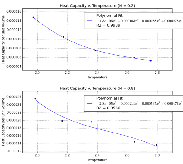
The general trend is that the specific heat capacity decreases as temperature increases. At higher temperatures, ${\left(\frac{\partial \ln Q}{\partial T}\right)}_V$ decreases and the internal energy function is less responsive to an increase in temperature.

NJ: Even though this is a classical system, we can think about the "modes" in which it can store heat. Your equation indicates that at high temperatures, the modes become more closely spaced in energy. It therefore requires less energy to "promote" the system to a higher energy state, so the heat capacity is lower.

At higher densities, the heat capacity per unit volume increases. In other words, heat capacity increases with the number of atoms. This is natural because the specific heat capacity is an extensive property that is proportional to the size of the system.

NJ: This is right, but remember that specific heat capacity is intensive. What you've worked out is just heat capacity, which is extensive.

Section 5: Structural Properties and The Radial Distribution Function

The Radial Distribution Function

All RDFs have the value of strictly zero in the region 0 to 0.75 units of length, implying that the repulsive forces really dominate in this region. RDFs generally oscillate around unity, although solid oscillations carry on much further than liquid. The solid lattice displays long-range order in the range simulated in the ensemble, meaning that it has periodic energetic interactions which continue to the edges of the box. As the crystal melts, some of its order is lost, and the liquid phase displays short-range order, up to its third-nearest neighbour. The distances of its neighbours stay roughly the same in liquid and solid phases. NJ: I don't think so. The small peaks count as neighbours as well!

When the liquid vapourises, the gas phase RDF suggests only one shell of atoms with high certainties. This effect is due to the minima of the attractive force, and the RDF sharply decreases as the shallow attractive component in the Lennard-Jones potential approaches zero. We can see that after $3.5\sigma$, the positions of individuals gaseous atoms are essentially random, which agrees with analysis on the Lennard-Jones potential in the earlier sections of this report.

The Solid Lattice

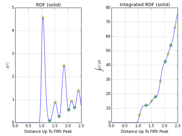
The peaks of the RDF itself represents the most likely distance to find these coordinating shells, and we shall use these distances, marked in yellow, as the mean distance between the central atom and its neighbours. After these peaks, the function sharply decreases due to repulsive forces from the atom's neighbours. The values of the integral at the distances where the RDF itself minimises are the cumulative coordination numbers of its neighbours within that distance. These values, marked in green, are 12.022, 17.958, and 42.224 corresponding to first three troughs. The implication is that the coordination numbers are 12, 6, and 24 for its most, 2nd-, and 3rd- nearest neighbours respectively.

Using the geometric arrangement of the face-centred lattice, we can relate the distances of its nearest neighbours to the size of the unit cell, which we defined as $l=1.49380$ units of length by setting the system number density to 0.8.

NJ: Careful, you set the number density to 1.2.

An illustration of the interatom distances in a face-centred cubic cell. The distances A, B, C, in the order from closest to furthest, are the three atoms closest to the atom in question. All atoms are equivalent to each other in our system. Not all members of the first three shells are represented.

The peaks for the solid RDF were extracted. In the same row, the mathematical relationship between the distance and unit cell length is given. Each of these peak r values can be used to calculate the unit cell length to evaluate if the simulation agrees with theoretical models.

Distance Peak	Geometric Relationship With $l$	$l$	Coordination Number
1.055	$\frac{\sqrt{2}}{2}l$	1.492	12
1.515	$l$	1.515	8
1.845	$\frac{\sqrt{6}}{2}l$	1.507	24

The coordination numbers match the connotations of the integrated RDF. The average unit cell length over its three nearest neighbours is $l=1.50467$, which is slightly higher than the original specification in which $l=1.49380$. Although they do agree, the fact that our finite-sized system gives a larger $l$ may be due to edge effects.

NJ: Lovely presentation. There could be a few things going on. You could have worked out a standard error for these three peaks to get some idea of "how close" you were to the initial value.

Section 6: Dynamical Properties and The Diffusion Coefficient

Mean Squared Displacement

In random Brownian motion, the position probability density diffuses out over time. Einstein hypothesised that the diffusion coefficient is proportional to the mean squared displacement of an ensemble of particles.

We have seen that the probability density function would not diffuse out for solid systems, as the lattice carries edges out to infinity. Therefore we would only expect to see random motion and a non-zero diffusion coefficient in liquid and gaseous systems. From the graphs, the gradient, and therefore the value of the diffusion coefficient of the solid systems are zero. The gradient becomes constant only after the system has equilibrated. I would take 2000 timesteps as the cutoff point, and extract the average gradient of the data beyond 2000 timesteps. $\text{Gradient}=\frac{1}{6}\times \frac{1}{\text{Timestep Used}}\times D$.

$D$ $({\text{Length}}^2{\text{ Time}}^{-1})$	8000 Atoms	One Million Atoms
solid	$0$	$0$
liquid	$6.7502\times 10^{-2}$	$7.0882\times 10^{-2}$
gas	$1.7699$	$2.4129$

Somewhat surprisingly, the gaseous MSD functions have an initial parabolic region. At short timescales, Einstein's description of the interactions between the atom and its surroundings breaks down. In our simulation, particles are given randomised velocity according to the Boltzmann distribution. In the initial region, the particles' initial inertia dominate the MSD function before its motion is changed by collisions with other particles. This effect is thought to exist for fluid states, i.e. gas and liquids, however, the high density of the liquid state means that the timescale during which the ballistic motion dominates is mush shorter.

In the solid state system, which is not described by Brownian motion, the initial region also differs greatly from the later, equilibrated region. The square displacement of the particle shoots up to some value and comes down rapidly, presumably due to restrictions of positions of individual atoms in a solid lattice. The kinetic energy is thoroughly dispersed, the oscillation randominises, and the mean squared displacement converges to 0.020 Length².

Quite noticeably the million-atom system suggests a much higher diffusion constant than the 8000-atom system. The principle of the finite system effect implies the diffusion constant of a real dynamic system is higher than the milllion-atom result.

NJ: It could be. It's most likely that you used different conditions to me for your vapour simulation though - I didn't tell you what I used.

Velocity Autocorrelation Function

VACF of A Harmonic Oscillator

The velocity of a harmonic oscillator is the derivative of its position function with respect to time,

$\begin{array}{rl}x(t)& =A\cos (\omega t+\varphi )\\ v(t)& =-A\omega \sin (\omega t+\varphi )\\ v(t+\tau )& =-A\omega \sin (\omega t+\omega \tau +\varphi )\end{array}$

Substituting $v(t)$ and $v(t+\tau )$ into the VACF equation,

$\begin{array}{rl}C(\tau )& =\frac{\underset{-\mathrm{\infty }}{\overset{\mathrm{\infty }}{\int }}v\left(t\right)v(t+\tau )\mathrm{d}t}{\underset{-\mathrm{\infty }}{\overset{\mathrm{\infty }}{\int }}{v}^2\left(t\right)\mathrm{d}t}\\ & =\frac{A^2{\omega }^2\underset{-\mathrm{\infty }}{\overset{\mathrm{\infty }}{\int }}\sin (\omega t+\varphi )\sin (\omega t+\omega \tau +\varphi )\mathrm{d}t}{A^2{\omega }^2\underset{-\mathrm{\infty }}{\overset{\mathrm{\infty }}{\int }}{\sin }^2(\omega t+\varphi )\mathrm{d}t}\\ \end{array}$

Using the product-to-sum formula $\sin a\sin b=\frac{1}{2}[\cos (a-b)-cos(a+b)]$,

$\begin{array}{rl}C(\tau )& =\frac{\underset{-\mathrm{\infty }}{\overset{\mathrm{\infty }}{\int }}\cos (\omega \tau )\mathrm{d}t-\underset{-\mathrm{\infty }}{\overset{\mathrm{\infty }}{\int }}\cos (2\omega t+\omega \tau +2\varphi )\mathrm{d}t}{2\underset{-\mathrm{\infty }}{\overset{\mathrm{\infty }}{\int }}{\sin }^2(\omega t+\varphi )\mathrm{d}t}\\ & \text{The first integral on the nominator is even and evaluates to zero,}\\ & =\frac{0-\underset{-\mathrm{\infty }}{\overset{\mathrm{\infty }}{\int }}\cos (2(\omega t+\varphi )+\omega \tau )\mathrm{d}t}{2\underset{-\mathrm{\infty }}{\overset{\mathrm{\infty }}{\int }}{\sin }^2(\omega t+\varphi )\mathrm{d}t}\end{array}$

For the nominator, we can use the product-to-sum identity $\cos (a+b)=\cos a\cos b-\sin a\sin b$ to cancel more even functions.

For the denominator, we can use the double angle formula for cosine to derive the power reduction formula ${\sin }^2(\theta )=\frac{1-\cos (2\theta )}{2}$.

$\begin{array}{rl}C(\tau )& =-\frac{\underset{-\mathrm{\infty }}{\overset{\mathrm{\infty }}{\int }}\cos (2(\omega t+\varphi )+\omega \tau )\mathrm{d}t}{2\underset{-\mathrm{\infty }}{\overset{\mathrm{\infty }}{\int }}{\sin }^2(\omega t+\varphi )\mathrm{d}t}\\ \\ & \text{After using product-to-sum formula on nominator,}\\ & =-\frac{\underset{-\mathrm{\infty }}{\overset{\mathrm{\infty }}{\int }}\cos (2(\omega t+\varphi ))\cos \left(\omega \tau \right)\mathrm{d}t+\underset{-\mathrm{\infty }}{\overset{\mathrm{\infty }}{\int }}\sin (\omega \tau )\sin (2(\omega t+\varphi ))\mathrm{d}t}{2\underset{-\mathrm{\infty }}{\overset{\mathrm{\infty }}{\int }}{\sin }^2(\omega t+\varphi )\mathrm{d}t}\\ & \text{After using power reduction formula on denominator,}\\ & =-\frac{\underset{-\mathrm{\infty }}{\overset{\mathrm{\infty }}{\int }}\cos (2(\omega t+\varphi ))\cos \left(\omega \tau \right)\mathrm{d}t+\underset{-\mathrm{\infty }}{\overset{\mathrm{\infty }}{\int }}\sin (\omega \tau )\sin (2(\omega t+\varphi ))\mathrm{d}t}{\underset{-\mathrm{\infty }}{\overset{\mathrm{\infty }}{\int }}\mathrm{d}t-\underset{-\mathrm{\infty }}{\overset{\mathrm{\infty }}{\int }}\cos (2(\omega t+\varphi ))\mathrm{d}t}\\ \\ & \text{Integrals of odd functions evaluate to zero:}\\ & =\frac{-\cos \left(\omega \tau \right)\underset{-\mathrm{\infty }}{\overset{\mathrm{\infty }}{\int }}\cos (2(\omega t+\varphi ))\mathrm{d}t}{-\underset{-\mathrm{\infty }}{\overset{\mathrm{\infty }}{\int }}\cos (2(\omega t+\varphi ))\mathrm{d}t}\\ C(\tau )& =cos(\omega \tau )\end{array}$

However, real systems differ greatly from the harmonic oscillator VACF.

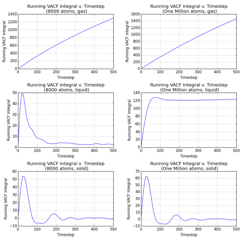
The VACF depicts damped harmonic oscillation, where the gaseous state VACF is the most damped, and the solid state VACF is the least damped. Evidently the harmonic oscillator takes into no consideration of other molecules, and is not damped by external motion at all. The gaseous overdamping is due to the low viscosity of the vapour state, as the system needs an very long time to exit the ballistic regime. The liquid VACF enters the Brownian motion regime at around the 1 time unit mark, and the initial inertia actually causes a slight correctional overshoot. Liquid has a greater viscosity than gas, and atom collisions therefore occur more frequently than the gas state. After the overshoot, the surrounding environment disperses and random motion begins. The solid lattice oscillates towards infinity like the classic harmonic oscillator because its equilibrium position is well-defined in the solid lattice. Any alterations to this position is quickly corrected to the equilibrium position because the interactions are very distance-sensitive in the high-density solid state and the surroundings do not disperse, unlike the liquid state. But still, the motion of the solid lattice does dampen, producing more randominised oscillations over time.

NJ: What is the significance of the minima?

VACF of Simulated Systems

D (Length2 Time-1)	8000 Atoms	One Million Atoms
solid	0	0
liquid	471.695	22522.9
gas	did not converge

We can see that the liquid diffusion constant is much higher than the calculations in the mean squared displacement gradients. The oscillating noise at the end of the liquid integral makes analysis difficult, and the running integral may seem to have converged by eye. But due to the discrepancy with the MSD values, the integral did not converge in this range of timesteps. One can imagine that the integral converges to the result of the desired order of magnitude after evaluating the running integral to a very vast number of timesteps. The million-atom simulation takes more timesteps to converge and suggests a much larger diffusion constant. Due to the time intensiveness of this approach, the VACF method is evidently not efficient in evaluating the diffusion constant using computer simulation. Even more evidently, the gaseous VACF integral fails to produce any convergence and implies an infinite diffusion constant, making it not suited to gaseous dynamics analysis.

NJ: I think something has gone wrong here. I think your "VACF Liquid 8000 atoms" integral might actually be for one of the solid systems. When you plotted the two sets of VACFs, you have a figure in which the solid and liquid values are mislabelled. NJ: Don't you have 5000 timesteps worth of output for the VACFs? Does the vapour still not converge?