Talk:Mod:csw114liquidsim

JC: General comments: Good report with all tasks answered and results well presented. Make sure you fully understand the background theory behind each task though so that you know exactly what the task is asking you and why.

Introduction to molecular reaction dynamics

TASK: Open the file HO.xls. In it, the velocity-Verlet algorithm is used to model the behaviour of a classical harmonic oscillator. Complete the three columns "ANALYTICAL", "ERROR", and "ENERGY": "ANALYTICAL" should contain the value of the classical solution for the position at time $t$, "ERROR" should contain the absolute difference between "ANALYTICAL" and the velocity-Verlet solution (i.e. ERROR should always be positive -- make sure you leave the half step rows blank!), and "ENERGY" should contain the total energy of the oscillator for the velocity-Verlet solution. Remember that the position of a classical harmonic oscillator is given by $x\left(t\right)=A\cos (\omega t+\varphi )$ (the values of $A$, $\omega$, and $\varphi$ are worked out for you in the sheet).

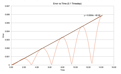
TASK: For the default timestep value, 0.1, estimate the positions of the maxima in the ERROR column as a function of time. Make a plot showing these values as a function of time, and fit an appropriate function to the data.

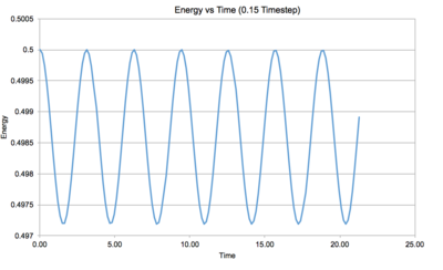
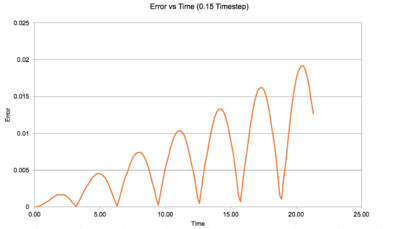
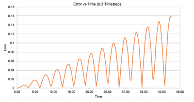
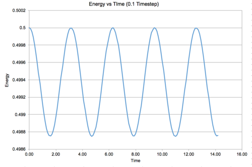
In this section of the experiment,the Veloctiy-Verlet algorithm was used to model the behaviour of a classical harmonic oscillator. From the data provided in the HO.xls files,the three columns "ANALYTICAL", "ERROR", and "ENERGY" were completed. The graphs below plots 1) displacement,2) total enery 3) absolute error between the classical and Verlet-Velocity derived solutions.

Displacement vs Time	Energy vs Time	Error vs Time
Displacement Vs Time	Energy vs Time	Error vs Time

The total energy of a classical harmonic oscillator was obtained by summing its potential and kinetic energy, according to the equation:

$\text{Total Energy}=U+K$
$\text{Total Energy}=\frac{1}{2}k{x}^2+\frac{1}{2}m{v}^2$

From the graphs shown above, we can see that displacement and energy display an oscillating behaviour while the error between the classical and Verlet-Velocity derived solutions increases over time
The position of the maxima in the error column were found and plotted as a function against time.

TASK: Experiment with different values of the timestep. What sort of a timestep do you need to use to ensure that the total energy does not change by more than 1% over the course of your "simulation"? Why do you think it is important to monitor the total energy of a physical system when modelling its behaviour numerically?
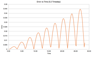
Several different timesteps were experimented with to observe its effects on the harmonic oscilator.

Timestep	Energy	Error
0.15	Energy Vs Time (0.15 Timestep)	Error Vs Time (0.15 Timestep)
0.20	Energy Vs Time (0.20 Timestep)	Error Vs Time (0.20 Timestep
0.30	Energy Vs Time (0.30 Timestep)	Error Vs Time (0.30Timestep

From the plots above, we can see that increasing the timestep for each simulation has the effect of increasing the amplitude and frequency of the oscillator. The error also increases as the timestep increases. This is because data is sampled at a less frequent rate, increasing the margin for error in the system as a result. We must monitor the total energy of a system to ensure that is obeying the law of energy conservation. By monitoring the total energy, we can monitor the equilibration process of the system.

JC: Did you decide which timestep gives you a variation in energy of less than 1? Why does the error oscillate over time?

Atomic Forces

TASK: For a single Lennard-Jones interaction, $\varphi \left(r\right)=4ϵ(\frac{{\sigma }^{12}}{r^{12}}-\frac{{\sigma }^6}{r^6})$, find the separation, $r_0$, at which the potential energy is zero. What is the force at this separation?

When modelling simple fluid systems, the Lennard Jones Potential is suitable to describe the interactions of atom pairs to a high degree of accuracy. The separation distance when potential energy = 0 occurs when $\sigma =r$. The force experienced at this distance is equivalent to ${\mathbf{F}}_i=\frac{24\epsilon }{\sigma }$(Workings shown in the table below)

Separation distance $r_0$

Force

$0=4\epsilon (\frac{{\sigma }^{12}}{r^{12}}-\frac{{\sigma }^6}{r^6})$ $0=(\frac{{\sigma }^{12}}{r^{12}}-\frac{{\sigma }^6}{r^6})$ $\frac{{\sigma }^{12}}{r^{12}}=\frac{{\sigma }^6}{r^6}$ ${\sigma }^6=r^6$ $\sigma =r$

${\mathbf{F}}_i=-\frac{\mathrm{d}\varphi \left(r\right)}{\mathrm{d}{\mathbf{r}}_i}$ ${\mathbf{F}}_i=-\frac{\mathrm{d}}{\mathrm{d}{\mathbf{r}}_i}4\epsilon (\frac{{\sigma }^{12}}{r^{12}}-\frac{{\sigma }^6}{r^6})$ ${\mathbf{F}}_i=\frac{24\epsilon }{r}{\left(\frac{\sigma }{r}\right)}^6[{\left(\frac{\sigma }{r}\right)}^2-1]$ ${\mathbf{F}}_i=\frac{24\epsilon }{r}{\left(\frac{\sigma }{r}\right)}^6[{\left(\frac{\sigma }{r}\right)}^2-1]$ when $\sigma =r$ ${\mathbf{F}}_i=\frac{24\epsilon }{\sigma }{\left(\frac{\sigma }{\sigma }\right)}^6[{\left(\frac{\sigma }{\sigma }\right)}^2-1]$ ${\mathbf{F}}_i=\frac{24\epsilon }{\sigma }$

TASK: Find the equilibrium separation, $r_{eq}$

At equilibrium separation, the attractive and repulsive forces balances out each other. This occurs when $F=0$. The equilibrium separation occurs at $r_{eq}=\sqrt[6]{2}\sigma$. The well depth at this separation was evaluated to be $\varphi \left(r_{eq}\right)=-ϵ$. (Working shown below)

Separation

Well Depth

${\mathbf{F}}_i=-\frac{\mathrm{d}\varphi \left(r\right)}{\mathrm{d}{\mathbf{r}}_i}$ ${\mathbf{F}}_i=-\frac{\mathrm{d}}{\mathrm{d}{\mathbf{r}}_i}4\epsilon (\frac{{\sigma }^{12}}{r^{12}}-\frac{{\sigma }^6}{r^6})$ $-4ϵ(-\frac{12{\sigma }^{12}}{r^{13}}+\frac{6{\sigma }^6}{r^7})=0$ $-\frac{12{\sigma }^{12}}{r^{13}}+\frac{6{\sigma }^6}{r^7}=0$ $-12{\sigma }^{12}+6{\sigma }^6{r}^6=0$ $r^6=2{\sigma }^6$ $r_{eq}=\sqrt[6]{2}\sigma$

$\varphi \left(r\right)=4ϵ(\frac{{\sigma }^{12}}{r^{12}}-\frac{{\sigma }^6}{r^6})$ $\varphi \left(r_{eq}\right)=4ϵ(\frac{{\sigma }^{12}}{(\sqrt[6]{2}\sigma {)}^{12}}-\frac{{\sigma }^6}{(\sqrt[6]{2}\sigma {)}^6})$ $\varphi \left(r_{eq}\right)=4ϵ(\frac{1}{4}-\frac{1}{2})$ $\varphi \left(r_{eq}\right)=-ϵ$

TASK: Evaluate the integrals $\underset{2\sigma }{\overset{\mathrm{\infty }}{\int }}\varphi \left(r\right)\mathrm{d}r$, $\underset{2.5\sigma }{\overset{\mathrm{\infty }}{\int }}\varphi \left(r\right)\mathrm{d}r$, and $\underset{3\sigma }{\overset{\mathrm{\infty }}{\int }}\varphi \left(r\right)\mathrm{d}r$ when $\sigma =ϵ=1.0$.

The Lennard Jones potential curve was evaluated for 3 sets of limits, each representing different seperation distances between two atoms.

$2\sigma -\mathrm{\infty }$	$2.5\sigma -\mathrm{\infty }$	$3\sigma -\mathrm{\infty }$
$\underset{2\sigma }{\overset{\mathrm{\infty }}{\int }}4ϵ(\frac{{\sigma }^{12}}{r^{12}}-\frac{{\sigma }^6}{r^6})\mathrm{d}r$ $4\epsilon [\frac{-{\sigma }^{12}}{11r^{11}}+\frac{{\sigma }^6}{5r^5}]$ $=4\epsilon \left(0\right)-4\epsilon (-\frac{{\sigma }^{12}}{11(2\sigma {)}^{11}}+\frac{{\sigma }^6}{5(2\sigma {)}^5})$ $=0-$ $4(-\frac{1}{11(2{)}^{11}}+\frac{1}{5(2{)}^5})$ $=0-0.024822$ $\approx -0.0248(3d.p.)$	$\underset{2\sigma }{\overset{\mathrm{\infty }}{\int }}4ϵ(\frac{{\sigma }^{12}}{r^{12}}-\frac{{\sigma }^6}{r^6})\mathrm{d}r$ $4\epsilon [\frac{-{\sigma }^{12}}{11r^{11}}+\frac{{\sigma }^6}{5r^5}]$ $=4\epsilon \left(0\right)-4\epsilon (-\frac{{\sigma }^{12}}{11(2.5\sigma {)}^{11}}+\frac{{\sigma }^6}{5(2.5\sigma {)}^5})$ $=0-$ $4(-\frac{1}{11(2.5{)}^{11}}+\frac{1}{5(2.5{)}^5})$ $=0-8.1767\times 10^{-3}$ $\approx -8.177\times 10^{-3}(3d.p.)$	$\underset{2\sigma }{\overset{\mathrm{\infty }}{\int }}4ϵ(\frac{{\sigma }^{12}}{r^{12}}-\frac{{\sigma }^6}{r^6})\mathrm{d}r$ $4\epsilon [\frac{-{\sigma }^{12}}{11r^{11}}+\frac{{\sigma }^6}{5r^5}]$ $=4\epsilon \left(0\right)-4\epsilon (-\frac{{\sigma }^{12}}{11(3\sigma {)}^{11}}+\frac{{\sigma }^6}{5(3\sigma {)}^5})$ $=0-$ $4(-\frac{1}{11(3{)}^{11}}+\frac{1}{5(3{)}^5})$ $=0-3.290\times 10^{-3}$ $\approx -3.290\times 10^{-3}(3d.p.)$

JC: Maths correct and well laid out.

Modelling realistic volumes of liquids

TASK: Estimate the number of water molecules in 1ml of water under standard conditions. Estimate the volume of $10000$ water molecules under standard conditions.
The number of water molecules in 1 mL of water under standard conditions were estimated.

Estimating number of H2O molecules in 1 mL
At 298K ${\rho }_{H_{2}O}=1gmo{l}^{-1}\approx \text{1 g}$ $\text{Number of mols}=\frac{1}{18.0}\approx \text{0.555 mols}$ $\text{N}=0.0555\times 6.023\times 10^{23}=3.346\times 10^{23}\text{molecules}$ $\text{N}=3.346\times 10^{23}\text{molecules}$ $\text{N}\approx 3.35\times 10^{23}\text{molecules}$

The volume of 10000 water molecules were evaluated as shown below:

Estimating volume of 10000 H2O molecules
$\text{Volume of 10000 molecules}=10000\times \frac{1}{3.346\times 10^{23}}$ $\text{V}=2.9885\times 10^{-19}\text{mL}$ $\text{V}\approx 2.99\times 10^{-19}\text{mL}$

JC: There should be 3x10^22 molecules of water in 1 ml, you are just out by a factor of 10, check your working. Volume of 10000 molecules is correct.

Periodic Boundary Function

TASK: Consider an atom at position $(0.5,0.5,0.5)$ in a cubic simulation box which runs from $(0,0,0)$ to $(1,1,1)$. In a single timestep, it moves along the vector $(0.7,0.6,0.2)$. At what point does it end up, after the periodic boundary conditions have been applied?.

Implementing a Periodic boundary function implies that when a particle interacts across a specified boundary , they can exit one end of the box and re-enter the other end. This enables the total number of particles in a box to stay constant. With the example shown below. The particle travels along a vector which would cause it to exit the box. However, instead of moving to the "next simulation box", the periodic boundary function stipulates that it "re-enters" the same simulated box via the opposite side, as demonstrated with its final position vector.

Position Vector
Position Vector before periodic boundary function = (0.5, 0.5, 0.5) + (0.7, 0.6, 0.2) = (1.2, 1.1, 0.7) Position Vector After periodic boundary function = (0.2, 0.1, 0.7)

JC: Correct.

Estimating Real Parameters for an Argon Atom

TASK: The Lennard-Jones parameters for argon are $$\begin{gathered} \sigma =0.34\mathrm{n}\mathrm{m},ϵ \\ / \\ {k}_B=120\mathrm{K} \end{gathered}$$. If the LJ cutoff is $r^{*}=3.2$, what is it in real units? What is the well depth in $$\begin{gathered} {\mathrm{k}\mathrm{J} \\ \mathrm{m}\mathrm{o}\mathrm{l}}^{-1} \end{gathered}$$? What is the reduced temperature $T^{*}=1.5$ in real units?

When working with the Lennard Jones potential, "reduced units" are often used to simplify mathematical calculations. Scaling factors are applied to experimental quantities to make expressions less cumbersome. In the exercise below, the real parameters for an Argon atom were calculated based on the reduced units provided.

Distance	Energy	Force
${\mathrm{r}}^{\mathrm{*}}=\frac{r}{\sigma }$ $\text{r}=3.2\times 0.34nm$ $\text{r}=1.08nm$	$E^{*}=\frac{E}{ϵ}$ $E^{*}=\frac{E}{ϵ}$ $\mathrm{s}\mathrm{i}\mathrm{n}\mathrm{c}\mathrm{e}\frac{ϵ}{k_B}=120K$ $ϵ=120K\times k_B$ $E=E*\times 120K\times k_B$ $E=0.9974{\text{kJ mol}}^{-1}$ $E\approx 0.9974{\text{kJ mol}}^{-1}$	$T^{*}=\frac{k_{B}T}{ϵ}$ $\frac{1}{T^{*}}=\frac{ϵ}{k_B}\times \frac{1}{T}$ $\frac{1}{T^{*}}=120\times \frac{1}{T}$ $\frac{1}{T^{*}}=\frac{1}{180}$ $T=180k$

JC: Good.

Equilibrium

Defining positions of atoms

TASK: Why do you think giving atoms random starting coordinates causes problems in simulations?

Giving atoms a random staring position would only introduce computational errors if the two atoms end up on the same starting position. This would affect the pairwise atomic interactions calculated by the Lennard Jones potential. If the atoms are superimposed on top of each other, it would imply a separation distance of 0, causing its potential to tend to $\mathrm{\infty }$. This would introduce errors when defining properties such as mass or velocity.

JC: If particles start too close together the high repulsion forces can make the simulation unstable and cause it to crash.

Creating a simulation box

TASK: Satisfy yourself that this lattice spacing corresponds to a number density of lattice points of $0.8$.
Consider instead a face-centred cubic lattice with a lattice point number density of 1.2. What is the side length of the cubic unit cell?
The simulation box used in this section of the experiment, has a lattice density of 0.8.
For a primative lattice structure with one atom per unit cell

$\rho =\frac{\text{Number of lattice points}}{\mathrm{V}\mathrm{o}\mathrm{l}\mathrm{u}\mathrm{m}\mathrm{e}}$
$\rho =\frac{1}{{(1.07722)}^3}$
$\rho =0.79999$
$\rho \approx 0.8$

For a FCC lattice with 4 atoms per unit cell and a number density of 1.2, the length of the unit cell was approximately 1.493. (Workings shown below)

$\rho =\frac{\text{Number of lattice points}}{{\left(\text{Length}\right)}^3}$
$1.2=\frac{1}{{(1.07722)}^3}$
${\left(Length\right)}^3=\frac{10}{3}$
$Length=1.49380$
$Length\approx 1.493\left(3dp\right)$


TASK: Consider again the face-centred cubic lattice from the previous task. How many atoms would be created by the create_atoms command if you had defined that lattice instead?

If a FCC lattice was used , 4000 atoms will be created as there are 4 lattice points per unit cell and the simulation box contains 1000 unit cells.

JC: Correct.

Setting properties of atoms

TASK: Using the LAMMPS manual, find the purpose of the following commands in the input script:

mass 1 1.0
pair_style lj/cut 3.0
pair_coeff * * 1.0 1.0

The following code used in simulations is related to the physical interactions between atoms.

Code	Purpose
mass 1 1.0	Defines the mass for all atoms of one or more atom type. Each atom is associated with a specific mass. In this simulation, atoms of type 1 are assigned a mass of 1.0.
pair_style lj/cut 3.0	It calculates the pairwise interactions between atoms using the Lennard-Jones potential. This line of code also defines an Rc term which specifies the global cutoff value for calculation of the potential at a distance of 3.0.
pair_coeff * * 1.0 1.0	This line of code calculates the force field coefficients in the Lennard Jones Potential. The "wildcard" asterisk is able to set coefficients for all pairs of atom interactions within the system. In this simulation the codes sets the force field constants for all pair wise interactions at 1.0

JC: What are the forcefield coefficients for the Lennard Jones potential? Why do we use a cutoff for the potential?

TASK: Given that we are specifying ${\mathbf{x}}_i\left(0\right)$ and ${\mathbf{v}}_i\left(0\right)$, which integration algorithm are we going to use? We are able to use the Velocity-verlet alogritym as we have defined $x_i\left(0\right)$ and $v_i\left(0\right)$.

Running the Simulation

TASK: Look at the first code below. what do you think the purpose of these lines is? Why not just write (second code)?

First code	Second code
### SPECIFY TIMESTEP ### variable timestep equal 0.001 variable n_steps equal floor(100/${timestep}) variable n_steps equal floor(100/0.001) timestep ${timestep} timestep 0.001<br> ### RUN SIMULATION ### run ${n_steps} run 100000	timestep 0.001 run 100000

The codes shown in the boxes can be used when running simulations of a system. Using the code in the first box allows us to vary the timestep of the simulation while running it for the same amount of time. It calculates the number of steps needed for the simulation to be ran within a fixed time. Although the number of steps taken will vary with timeset but it is within a fixed time frame.
The code in the second box will also allow us to vary the timestep but under slightly different conditions. This code would change the run time of the simulation and does not calculate the number of steps needed to be taken to run the simulation for a fixed time frame.

JC: Both pieces of code will run the same simulation, but the advantage of using variables as in the first case is that if we change the timestep, all properties which depend on the value of the timestep are also changed automatically.

Checking Equilibration

TASK: make plots of the energy, temperature, and pressure, against time for the 0.001 timestep experiment (attach a picture to your report). Does the simulation reach equilibrium? How long does this take? When you have done this, make a single plot which shows the energy versus time for all of the timesteps (again, attach a picture to your report). Choosing a timestep is a balancing act: the shorter the timestep, the more accurately the results of your simulation will reflect the physical reality; short timesteps, however, mean that the same number of simulation steps cover a shorter amount of actual time, and this is very unhelpful if the process you want to study requires observation over a long time. Of the five timesteps that you used, which is the largest to give acceptable results? Which one of the five is a particularly bad choice? Why?

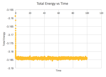
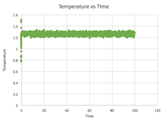
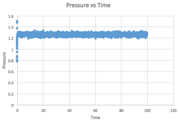
The thermodynamics output of the "melt crystal" simulations were analysed. The simulation was ran at a timestep of 0.01.Graphs of energy, temperature and pressure against times are plotted and shown below:

Total Energy vs Time	Temperature vs Time	Pressure vs Time

From the graphs, we see see that the system reaches equilibrium as the output can be seen fluctuating around a constant value. It can be seen that the system reaches equilibrium around 0.3 to 0.4.

Several simulations were ran at different time steps, a plot of total energy of each system vs time is shown in the graph below

Total energy vs Time (At different timesteps)

As the time step decreases, the total number of steps taken in the simulation increases. From the data, we can see that total energy for a timestep =0.015, increases with time and diverges. The system has not reached equilibrium and will not provide useful information can be gathered.It breaking the law of conservation of mass and is an indication that there are errors within the simulation.
With the 4 other timesteps chosen, it can be seen that total energy decreases over time and slowly begins to fluctuation around an equilibrium value.
With a smaller timestep chosen the accuracy of calculations increase. This would imply that among the 5 simulations ran, a timestep of 0.001 would provide the most accurate physical data regarding our system under consideration. However, it would be computationally very expensive. On the other hand a timestep of 0.0025 would provide a good balance, providing accuracy whilst giving us a reasonable time to monitor the system. The data obtained at a timestep of 0.0025 shows that it provides comparable output data in relation to a timestep of 0.001.

JC: The largest timestep doesn't conserve energy, but mass is unaffected by the timestep. The average total energy should not depend on the choice of timestep, as it does for 0.01 and 0.0075, so the best choice is 0.0025.

Running simulations under specific conditions

Thermostats and Barostats

TASK: We need to choose $\gamma$ so that the temperature is correct $T=\mathfrak{𝔗}$ if we multiply every velocity $\gamma$.Solve these to determine $\gamma$.
The temperature of the system can be controlled by multiplying it with a constant factor $\gamma$.
In the calculations below, a value of $\gamma$ has been calculated to ensure that the instantaneous temperature (T) is equivalent to the target temperature $\mathfrak{𝔗}$.

$E_K=\frac{3}{2}N{k}_{B}T$

$\frac{1}{2}\sum _i{m}_i{v}_i^2=\frac{3}{2}N{k}_{B}T$
Multiplying every velocity by gamma

$\frac{1}{2}\sum _i{m}_i{(v_i*\gamma )}^2=\frac{3}{2}N{k}_B\mathfrak{𝔗}$
$\frac{1}{2}\sum _i{m}_i{v}_i^2{\gamma }^2=\frac{3}{2}N{k}_B\mathfrak{𝔗}$
${\gamma }^2=\frac{\frac{3}{2}N{k}_B\mathfrak{𝔗}}{\frac{1}{2}\sum _i{m}_i{v}_i^{2}T}$
$\gamma =\pm \sqrt{\frac{\mathfrak{𝔗}}{T}}$

JC: Correct, gamma is the positive root as we don't want to change the direction of the particles velocity, just scale the magnitude of the velocity.

Examining the Input Script

TASK: Use the manual page to find out the importance of the three numbers 100 1000 100000. How often will values of the temperature, etc., be sampled for the average? How many measurements contribute to the average? Looking to the following line, how much time will you simulate?
The following lines of code were used to run the simulation.

Input code
fix aves all ave/time 100 1000 100000 v_dens v_temp v_press v_dens2 v_temp2 v_press2<br> run 100000

The first value 100 stipulates that the simulation will calculate average thermodynamic data with a space of every 100 timesteps. The second value 1000 causes the simulation to use 1000 data points to calculate the thermodynamic values. The third value,10,000, refers to the total number of timesteps to be used in the simulation. With a timestep of 0.0025 and 10000 steps will result in a simulation time of 250.

Equation of State

TASK: Choose 5 temperatures (above the critical temperature $T^{*}=1.5$), and two pressures (you can get a good idea of what a reasonable pressure is in Lennard-Jones units by looking at the average pressure of your simulations from the last section). This gives ten phase points — five temperatures at each pressure. Create 10 copies of npt.in, and modify each to run a simulation at one of your chosen $(p,T)$ points. You should be able to use the results of the previous section to choose a timestep. Submit these ten jobs to the HPC portal. While you wait for them to finish, you should read the next section.

TASK: Use software of your choice to plot the density as a function of temperature for both of the pressures that you simulated. Your graph(s) should include error bars in both the x and y directions. You should also include a line corresponding to the density predicted by the ideal gas law at that pressure. Is your simulated density lower or higher? Justify this. Does the discrepancy increase or decrease with pressure?

Variable	Values
Pressure	2.45 , 2.75
Temperature	1.6, 1.8, 2.0, 2.2, 2.4
Timestep	0.0025

In this section of the experiment, the isobaric-isothermal ensemble is used to calculate the equation of state This produced a set of 10 data points which are plotted in the graph shown below. The ideal gas equation was also used to 'predict' the density at each given temperature.

Pressure = 2.75	Pressure = 2.45

We can see that the ideal gas law predicts a higher density value compared to calculated values as it does not take into account inter-atomic interactions. The ideal gas law treats atoms as randomly moving points without any volume. It assumes that there are no repulsive interactions between atoms. Atoms would be closer together in comparison to the Lennard Jones potential model as they are not repelling each other. This leads to a higher calculated density as there are more atoms per unit area (in the ideal gas model).
On the other hand, the calculated densities are derived using the Lennard Jones potential and takes into account attractive and repulsive forces between atoms, resulting in deviations between the predicted and calculated densities. The ideal gas equation is only useful for modelling real fluidic systems at low densities where there are minimal atom interactions.

JC: Correct, how does the discrepancy between the ideal gas and simulation results change with pressure and temperature? Plot all of the data on one graph to see the trends more clearly.

Calculating Heat Capacities using statistical physics

TASK: As in the last section, you need to run simulations at ten phase points. In this section, we will be in density-temperature $({\rho }^{*},T^{*})$ phase space, rather than pressure-temperature phase space. The two densities required at $0.2$ and $0.8$, and the temperature range is $2.0,2.2,2.4,2.6,2.8$. Plot $C_V/V$ as a function of temperature, where $V$ is the volume of the simulation cell, for both of your densities (on the same graph). Is the trend the one you would expect? Attach an example of one of your input scripts to your report.

Heat capacity refers to the amount of energy needed to raise the temperature of a system by 1k.
In this section, the heat capacities were plotted as a function of time to produce a total of 10 data points as shown in the graph below. The simulation conditions used are shown in the table on the right

Variable	Values
Density	0.2,0.8
Temperature	2.0, 2.2, 2.4, 2.6, 2.8
Atoms	3375

Total energy vs Time (At different timesteps)

From the graph, we can see that increasing the temperature leads to a decrease in heat capacity. As the temperature of the system increases, it is possible to excite the particles to a higher energy level. However, as the higher energy states become increasingly populated, it becomes harder for the system to absorb more energy, thus leading to a lower specific heat capacity
From the graph, we can also see that density is proportional to heat capacity. Increasing the density of a system increases the number of atoms per unit cell. This increases the number of accessible mirco-states. The system is able to absorb more energy per unit cell, thus leading to a higher heat capacity. This also shows that heat capacity is an extensive property.

It can be inferred that the system has a finite number of energy levels as the heat capacity has not reached a constant value.

JC: Remember that your simulations are classical so there are no discrete energy levels. Why did you choose to fit your data with the line shown in the graph?

Input code

The following input code was used to calculate the heat capacity

Input code

#### DEFINE SIMULATION BOX GEOMETRY ### variable density equal 0.2 lattice sc ${density} region box block 0 15 0 15 0 15 create_box 1 box create_atoms 1 box ### DEFINE PHYSICAL PROPERTIES OF ATOMS ### mass 1 1.0 pair_style lj/cut/opt 3.0 pair_coeff 1 1 1.0 1.0 neighbor 2.0 bin ### SPECIFY THE REQUIRED THERMODYNAMIC STATE ### variable T equal 2.0 variable p equal 2.6 variable timestep equal 0.0025 ### ASSIGN ATOMIC VELOCITIES ### velocity all create ${T} 12345 dist gaussian rot yes mom yes ### SPECIFY ENSEMBLE ### timestep ${timestep} fix nve all nve ### THERMODYNAMIC OUTPUT CONTROL ### thermo_style custom time etotal temp press thermo 10 ### RECORD TRAJECTORY ### dump traj all custom 1000 output-1 id x y z ### SPECIFY TIMESTEP ### ### RUN SIMULATION TO MELT CRYSTAL ### run 10000 unfix nve reset_timestep 0 ### BRING SYSTEM TO REQUIRED STATE ### variable tdamp equal ${timestep}*100 fix nvt all nvt temp ${T} ${T} ${tdamp} run 10000 unfix nvt fix nve all nve reset_timestep 0 thermo_style custom step etotal temp atoms vol density variable energy equal etotal variable energy2 equal etotal*etotal variable temp equal temp variable temp2 equal temp*temp variable N equal atom variable N2 equal atoms*atoms variable vol equal vol variable density equal density fix aves all ave/time 100 1000 100000 v_energy v_energy2 v_temp v_temp2 v_density run 100000 variable T2 equal f_aves[4] variable tempave equal f_aves[3] variable E2 equal f_aves[1]*f_aves[1] variable EE equal f_aves[2] variable top equal ${EE}-${E2} variable heatcap equal (${top}/${T2})*${N2} variable heatcapvol equal ${heatcap}/vol print "Here are the results from this calculation!! " print "--------" print "Temperature: ${tempave}" print "Heat Capacty/Vol: ${heatcapvol}" print "Heat Capacty: ${heatcap}"

Structural properties and the radial distribution function

TASK: perform simulations of the Lennard-Jones system in the three phases. When each is complete, download the trajectory and calculate $g(r)\text{ and }\int g(r)\mathrm{d}r$. Plot the RDFs for the three systems on the same axes, and attach a copy to your report. Discuss qualitatively the differences between the three RDFs, and what this tells you about the structure of the system in each phase. In the solid case, illustrate which lattice sites the first three peaks correspond to. What is the lattice spacing? What is the coordination number for each of the first three peaks?

Phase	Temperature	Density
Solid	1.2	1.1
Liquid	1.2	0.8
Gas	1.2	0.1

Data on the structure of the Lenard Jones system can be characterised by its radial distribution function. In this section of the experiment, the radial distribution functions $g(r)$ were calculated for the solid, liquid, and vapour phases . Plots of $g(r)\text{ and }\int g(r)\mathrm{d}r$ are shown below. Simulation conditions are provided on the right. A timestep of 0.002 was used to perform this set of simulations.

$g\left(r\right)$ vs distance	$\int g\left(r\right)$ vs distance

A peak indicates a favoured separation distance for the neighbours from a reference atom. The number of peaks in each radial distribution function decreases in the following manner : Solid> Liquid >Gas.

• Gas Phase

The rdf of the Gas phase shows one main peak before it decays to a value of one as the distance r increases. Structurally, the Gaseous phase lacks a regular structure thus heavily influencing its rdf. It also suggest that it only has one coordination sphere surrounding the reference atom. The peak present for the gaseous states is significantly broadened possibly due to the thermal motion of the atoms.

• Liquid Phase

The rdf of the liquid phase shows a fewer number of peaks compared to the solid phase. This is because there is local ordering within the liquid phase but no long range order. The first peak in the rdf is the highest, indicating that the reference atom experiences the strongst attractive and repulsive interactions with its nearest neighbour.

• Solid Phase

The rdf of the Solid phase shows multiple peaks even as the distance increases. This is because Solids display long range order where atoms are arranged in a orderly manner. Each peak on the rdf of the solid phase corresponds to the atoms 'nearest neighbour, with the first peak corresponding to the first nearest neighbours, second peak corresponding to the second nearest neighbour etc.
For a face centered cubic lattice, with a lattice parameter "a" and unit cell length of 1.49380, the distance of its neighbours were calculated and compared to experimental values as shown in the table below:

Peak Number	Lattice Spacing (Theoratical)	Lattice Spacing (Calculations)	Coordination Number
1 (Nearest Neighbour)	$\frac{\sqrt{2}}{2}a==1.06\text{ (3sf) }$	1.025	12
2 (Second Nearest Neighbour)	$a=1.49\text{ (3sf) }$	1.457	6
3 (Third Nearest Neighbour)	$\frac{\sqrt{6}}{2}a=1.83\text{ (3sf) }$	1.825	24

A zoomed in version of the radial distribution function for the solid simulation is shown below. The distances between the reference atom and its 3 nearest neighbors are indicated on the graph.

Radial Distribution Function Solid Phase

JC: Good description of the solid, liquid and gas RDFs. The lattice spacing is the width of the unit cell, not the distance to the first nearest neighbour in an fcc lattice, what do the results in your table show? How did you calculate the coordination numbers for the first three peaks? Showing the atoms responsible for these peaks on a diagram of an fcc lattice would have been good.

Dynamical properties and the diffusion coefficient

Mean Squared Displacement

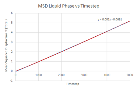
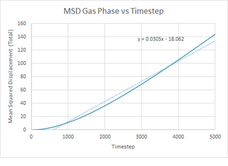
TASK: make a plot for each of your simulations (solid, liquid, and gas), showing the mean squared displacement (the "total" MSD) as a function of timestep. Are these as you would expect? Estimate D in each case. Be careful with the units! Repeat this procedure for the MSD data that you were given from the one million atom simulations.

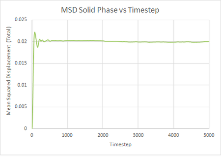
The mean squared displacements of small and large systems were studied for the solid, liquid and gaseous phase. This was plotted as a function against time and shown below:

Phase	Mean Squared Displacement (Total) - Small Systems	Mean Squared Displacement (Total) - Large Systems
Solid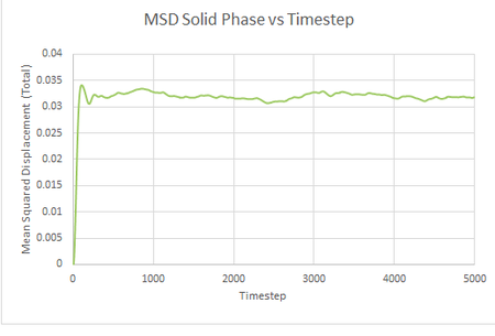
Liquid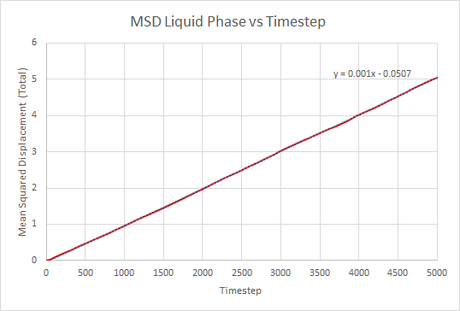
Gas

From the graphs showing Mean Squared Distance against timestep, the diffusion coefficient for each system can be estimated using the following equation $\text{D}=\frac{1}{6}\frac{\partial ⟨r^2\left(t\right)⟩}{\partial t}$.The diffusion coefficients were estimated for each system and shown in the table below:

Phase	Diffusion Coefficent - Small Systems	Diffusion Coefficient - Large Systems
Solid	$\approx 0$	$\approx 0$
Liquid	$\text{D}=\frac{1}{6}\times \frac{4.0226-1.97381}{2000\times 0.002}=0.085$	$\text{D}=\frac{1}{6}\times \frac{4.1237-2.00809}{2000\times 0.002}=0.0820$
Gas	$\text{D}=\frac{1}{6}\times \frac{64.2573-25.760}{2000\times 0.002}=1.60$	$\text{D}=\frac{1}{6}\times \frac{105.541-36.398}{2000\times 0.002}=2.88$

From the table, we can see that the diffusion coefficient increases in the following order: Solid , Liquid. Gas.
The diffusion coefficient of the solid phase is negligible as the atoms are held in fixed positions. The diffusion coefficients for the Liquid and Gaseous phases increase with time. In these two phases, the atoms are no longer held in fixed positions and have greater molecular motion. The gaseous phase shows a higher diffusion coefficient compared to the liquid phase. This is due to the difference in densities between the two states. In the gaseous phase, molecules have a greater mean free path and can travel a further distance before colliding with another molecule. Moreover, atoms in the gaseous phase experience weaker intermolecular forces and are able to move with a greater degree of freedom.

The simulation was also repeated for large systems containing one million atoms and the results are similar to the results obtained from simulations of small systems

JC: To calculate D you should only fit a straight line to the linear part of the MSD graph as this is the diffusive regime, not the whole data set. Why is the gas MSD graph curved at short times?

Velocity Autocorrelation Function

TASK: In the theoretical section at the beginning, the equation for the evolution of the position of a 1D harmonic oscillator as a function of time was given. Using this, evaluate the normalised velocity autocorrelation function for a 1D harmonic oscillator
The normalised velocity autocorrelation function for a 1D harmonic oscillator is evaluated.

VACF of the 1D Harmonic Oscilator.

$\text{ Since }x(t)=A\cos (\omega t+\varphi )$ $v(t)=\frac{\mathrm{d}x(t)}{\mathrm{d}t}=-A\omega \sin (\omega t+\varphi )$ $C\left(\tau \right)=\frac{\underset{-\mathrm{\infty }}{\overset{\mathrm{\infty }}{\int }}-\omega A\sin (\omega t+\varphi )\times -\omega A\sin (\omega (t+\tau )+\varphi )\mathrm{d}t}{\underset{-\mathrm{\infty }}{\overset{\mathrm{\infty }}{\int }}{\omega }^2{A}^2{\sin }^2(\omega t+\varphi )\mathrm{d}t}$ $C\left(\tau \right)=\frac{\underset{-\mathrm{\infty }}{\overset{\mathrm{\infty }}{\int }}\sin (\omega t+\varphi )\times \sin (\omega t+\tau +\varphi )\mathrm{d}t}{\underset{-\mathrm{\infty }}{\overset{\mathrm{\infty }}{\int }}{\sin }^2(\omega t+\varphi )\mathrm{d}t}$ $\text{Using the identity}\sin (A+B)=\sin \left(A\right)\cos \left(B\right)+\sin \left(A\right)\cos \left(B\right)$ $\text{Where }(\omega t+\varphi )=\text{ and }\omega \tau =B$ $C\left(\tau \right)=\frac{\underset{-\mathrm{\infty }}{\overset{\mathrm{\infty }}{\int }}\sin (\omega t+\varphi )\times \sin (\omega t+\varphi )\cos \left(\omega \tau \right)\mathrm{d}t+\underset{-\mathrm{\infty }}{\overset{\mathrm{\infty }}{\int }}\sin (\omega t+\varphi )\sin \left(\omega \tau \right)\cos (\omega t+\varphi )\mathrm{d}t}{\underset{-\mathrm{\infty }}{\overset{\mathrm{\infty }}{\int }}{\sin }^2(\omega t+\varphi )\mathrm{d}t}$ $\cos \left(\omega \tau \right)\text{ and }\sin \left(\omega \tau \right)\text{ have a constant value }$ $C\left(\tau \right)=\cos \left(\omega \tau \right)\frac{\underset{-\mathrm{\infty }}{\overset{\mathrm{\infty }}{\int }}{\sin }^2(\omega t+\varphi )}{\underset{-\mathrm{\infty }}{\overset{\mathrm{\infty }}{\int }}{\sin }^2(\omega t+\varphi )}\times \sin \left(\omega \tau \right)\frac{\underset{-\mathrm{\infty }}{\overset{\mathrm{\infty }}{\int }}\sin (\omega t+\varphi )\times \cos (\omega t+\varphi )\mathrm{d}t}{\underset{-\mathrm{\infty }}{\overset{\mathrm{\infty }}{\int }}{\sin }^2(\omega t+\varphi )\mathrm{d}t}$ $C\left(\tau \right)=\cos \omega \tau +\frac{\sin \omega \tau {\left[{\sin }^{}(\omega t+\varphi )\right]}_{-\mathrm{\infty }}^{\mathrm{\infty }}}{2\omega \underset{-\mathrm{\infty }}{\overset{\mathrm{\infty }}{\int }}{\sin }^2(\omega t+\varphi )\mathrm{d}t}$ $C\left(\tau \right)=\cos \omega \tau$

JC: Correct result, but the integral of cos(t)xsin(t) is not sin^2(t) in the last but one line. cos(t)xsin(t) is an odd function so the integral from -inf to inf will be zero.

On the same graph, with x range 0 to 500, plot $C\left(\tau \right)$ with $\omega =1/2\pi$ and the VACFs from your liquid and solid simulations. What do the minima in the VACFs for the liquid and solid system represent? Discuss the origin of the differences between the liquid and solid VACFs. The harmonic oscillator VACF is very different to the Lennard Jones solid and liquid. Why is this? Attach a copy of your plot to your writeup.

The velocity autocorrelation function of both Solid and Liquid simulations as well as the approximation from the 1 dimensional harmonic oscillator are plotted in the graph shown below:

Velocity Auto-correlation Function vs Timestep

The mimimas in the VACFs for the solid and liquid systems indicate that the velocities of the atoms are reversed
The VACFs for the solid and liquid phase show the behavior of a dampened oscillator. They do not display perfect oscillatory behaviour due to frictional forces which causes it to oscillate with a frequency and amplitude that decreases over time. In the solid phase, atoms are held in fixed positions and can interact with neighboring atoms. In the liquid phase, atoms are no longer held in fixed positions and are able to move around more freely to interact with other atoms. The increased motion in the liquid phase has an increases dampening effect on its oscillatory behavior. As such, the VACF for the liquid phase decays at a much quicker rate compared to the solid phase.
The VACF for the Harmonic oscillator represents a situation where there are no interactions to dampen oscillatory motion. It oscillates with only the restoring force acting on the system.The velocity goes in the reverse direction at the end of each oscillation. The VACF does not decay unlike the phases modelled using the Lennard-Jones potential.

JC: What do you mean by frictional forces? The VACF decays because of collisions between particles.

TASK: Use the trapezium rule to approximate the integral under the velocity autocorrelation function for the solid, liquid, and gas, and use these values to estimate $D$ in each case. You should make a plot of the running integral in each case. Are they as you expect? Repeat this procedure for the VACF data that you were given from the one million atom simulations. What do you think is the largest source of error in your estimates of D from the VACF?

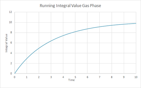
The trapezium rule was used to estimate the integral under the VACF for the solid liquid and gaseous phase. The calculation was also performed on a simulation of one million atoms. The plots are shown in the table below.

Phase	Running Integral Value - Small Systems	Running Integral Value - Large Systems
Solid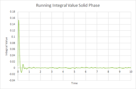
Liquid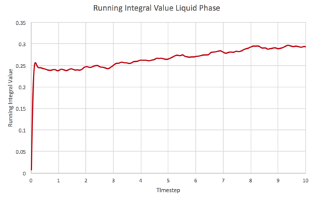
Gas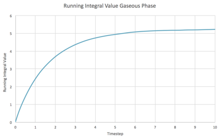

From the graphs, the diffusion coefficient for each system can be estimated using the following equation $D=\frac{1}{3}\underset{0}{\overset{\mathrm{\infty }}{\int }}\mathrm{d}\tau ⟨\mathbf{v}\left(0\right)\cdot \mathbf{v}\left(\tau \right)⟩$The diffusion coefficients were estimated for each system and shown in the table below:

Phase	Diffusion Coefficent - Small Systems	Diffusion Coefficient - Large Systems
Solid	$\text{D}=\frac{1}{3}\times 0.000523=0.000174\text{ 3sf }$	$\text{D}=\frac{1}{3}\times 0.0001364=4.54\text{x}10^{-5}\text{ 3sf }$
Liquid	$\text{D}=\frac{1}{3}\times 0.29364=0.0979\text{ 3sf }$	$\text{D}=\frac{1}{3}\times 0.27028=0.0901\text{ 3sf }$
Gas	$\text{D}=\frac{1}{3}\times 5.23060=1.74\text{ 3sf }$	$\text{D}=\frac{1}{3}\times 9.80553=3.27\text{ 3sf }$

The diffusion coefficients obtained by approximating the area under the VACF integrals show a similar trend to the diffusion coefficients obtained from the MSD graphs. One source of error when estimating the diffusion coefficient from the VACF would be an ineffective trapezium approximation to the VACF curves. In the future, smaller timesteps could use used. This would provide a better estimation for the area under the integral by producing a better trapezium approximation.

However, the greatest source of error while running the VACF simulation would be the amount of time units simulated when running the simulation. From the running integral graphs, we can see that the liquid and gaseous phases have not reached equilibrium and its value is still increasing. Running the simulation for a longer time would allow it to reach equilibrium and lead to a better estimation of diffusion coefficient values.

JC: Good.