Talk:Mod:am6913LS

Liquid Simulations Computational Lab

Introduction to Molecular Dynamics Simulation

Tasks 1 and 2

In the HO.xls file, the three columns were completed.

'ANALYTICAL' showed the values for the position at time t, computed classically using the steady state equation for the harmonic oscillator

$x\left(t\right)=A\cos (\omega t+\varphi )$. Here $A=1$, $\omega =1$ and $\varphi =0$

Initially, the timestep was set at 0.1.

The graph shown below demonstrates that the results for the above harmonic oscillator equation, shown by an blue line, agree with the results from the velocity-Verlet algorithm, shown by red dots.

Figure 1: Harmonic Oscillator and the Velocity-Verlet Algorithm vs. Time at 0.1 Timestep

'ERROR' calculated the absolute difference between the positions found classically in 'ANALYTICAL' and those found using the velocity-Verlet algorithm. It can be seen in figure 2 that the error varies periodically and gets larger with time. In figure 3 the maxima of each peak were found and isolated to produce a graph following a linear function. The gradient of this line was +0.0004, reflecting the fact that the maxima gain amplitude during the trajectory. The observed trend occurs due to the fact that the velocity-Verlet algorithm is based on an iteration; as the calculation progresses, errors accumulate over time and will therefore continue to increase throughout the simulation.

NJ: Good

Figure 2: Error vs. Time at 0.1 Timestep

Figure 3: Max Error vs. Time at 0.1 Timestep

'ENERGY' used the equation E = ½mv² + ½kx² to find the total energy of the oscillator for the velocity-Verlet solution. Since the system is approximated by a simple harmonic oscillator in which the atoms compress and extend due to the conversion between kinetic and potential energy, the total energy remains constant and there is no exchange/energy losses to the surroundings. In figure 4, we can see that the system follows a sinusoidal function that fluctuates about an average energy value of 0.499. Since at a timestep of 0.1 the fluctuations have a range of 0.0013, the energy only changes by 0.13% of the average in either direction.

NJ: Good. Why do you think this is?

Figure 4: Energy vs. Time at 0.1 Timestep

Given that $\omega =\sqrt{\frac{k}{\mu }}$, you would expect that an increase in mass would result in a smaller vibration frequency (as the reduced mass would also increase) and hence a periodic function with a larger wavelength, whilst increasing the force constant, k, would have the opposite effect.

Task 3

By changing the values of the timestep, it became clear that decreasing its value gave a smaller energy dispersion and fewer fluctuations per unit time, whilst increasing had the opposite effect. Hence, by increasing the timestep to 0.2, the total energy did not change by more than 1% over the course of the simulation; this was found by comparing 1% of the average value of the fluctuations with the difference between the maximum and minimum of the curve. At a timestep of 0.2, these values came to 0.005 and 0.00498 respectively.

It is important to monitor the total energy of a physical system to ensure that the simulation is obeying the law of conservation of energy and fluctuates about a constant, average energy. NJ: Good Smaller fluctuations lead to a better-defined average value. NJ: That's not quite true - it just means that the standard deviation is smaller.

Task 4

Using the equation for a single Lennard-Jones interaction:

$\varphi \left(r\right)=4ϵ(\frac{{\sigma }^{12}}{r^{12}}-\frac{{\sigma }^6}{r^6})$

Where $r^{12}$ is the short range repulsion and $r^6$ is the long range attraction between the two atoms.

The separation at which the potential energy is zero was found by setting $\varphi \left(r\right)=0$. This gave $r_0=\sigma$ as the attraction and repulsion cancel out.

The corresponding force was calculated by finding $\mathbf{F}=-\frac{\varphi \left(r\right)}{\mathrm{d}\mathbf{r}}$ and substituting $r_0=\sigma$:

$\mathbf{F}=-\frac{\varphi \left(r\right)}{\mathrm{d}{\mathbf{r}}_i}=4ϵ(12{\sigma }^{12}{r}^{-13}-6{\sigma }^6{r}^{-7})$ $\mathbf{F}(r_0)=\frac{24ϵ}{\sigma }$

The equilibrium separation was found by setting $\mathbf{F}=-\frac{\varphi \left(r\right)}{\mathrm{d}\mathbf{r}}=0$. This gave $r_{eq}=2^{\frac{1}{6}}\sigma$ as $\frac{12{\sigma }^{12}}{r^{13}}=\frac{6{\sigma }^6}{r^7}$.

The resulting well depth was calculated by:

$\varphi \left(r_{eq}\right)=4ϵ(\frac{{\sigma }^{12}}{(2^{\frac{1}{6}}\sigma {)}^{12}}-\frac{{\sigma }^6}{(2^{\frac{1}{6}}\sigma {)}^6})$ $\varphi \left(r_{eq}\right)=4ϵ(\frac{1}{4}-\frac{1}{2})$ $\varphi \left(r_{eq}\right)=-ϵ$

Finally the following integrals were evaluated for $\sigma =ϵ=1.0$:

$\underset{2\sigma }{\overset{\mathrm{\infty }}{\int }}\varphi \left(r\right)\mathrm{d}r=4ϵ{[-\frac{1}{11}{\sigma }^{12}{r}^{-11}+\frac{1}{5}{\sigma }^6{r}^{-5}]}_{2\sigma }^{\mathrm{\infty }}=-0.025$

$\underset{2.5\sigma }{\overset{\mathrm{\infty }}{\int }}\varphi \left(r\right)\mathrm{d}r=-0.008$

$\underset{3\sigma }{\overset{\mathrm{\infty }}{\int }}\varphi \left(r\right)\mathrm{d}r=-0.003$

Task 5

Given that the density of water under standard conditions is $\rho =999.972kg.m^{-3}$ and its molar mass is $M_r=18g.mo{l}^{-1}$, then the number of molecules of water in 1mL is:

$\rho =1.00g.c{m}^{-3}$ and $m_{H_{2}O}=1.00g$ $\frac{1.00g}{18g.mo{l}^{-1}}=0.056mol$ $0.056mol*6.022*10^{23}=3.35*10^{22}$

If there were 10,000 molecules of water, they would occupy a volume of 3.0 x 10^-19mL (by doing the reverse of the above calculation) NJ: Show your working for this too

Task 6

An atom starting at position $(0.5,0.5,0.5)$ in a cubic simulation box under periodic boundary conditions will end up at point $(0.2,0.1,0.7)$ after the simulation has run from $(0,0,0)$ to $(1,1,1)$ along the vector $(0.7,0.6,0.2)$.

Where periodic boundary conditions not adopted, then the atom would have ended at the point $(1.2,1.1,0.7)$

Task 7

Given that the Lennard-Jones parameters for argon are:

$\sigma =0.34\mathrm{n}\mathrm{m}$ and $\frac{ϵ}{k_B}=120K$

The LJ cutoff of $r^{*}=3.2$ can be converted using $r^{*}=\frac{r}{\sigma }$ to give $r=1.09nm$ in real units.

The well depth can be calculated using $ϵ=120K*k_B$ to give $$\begin{gathered} ϵ=1.66*10^{-21}J=1.00{kJ \\ mol}^{-1} \end{gathered}$$

The reduced temperature of $T^{*}=1.5$ can be converted using $T^{*}=\frac{k_{B}T}{ϵ}$ to give $T=180K$ in real units.

NJ: Good, this section is all correct and nicely presented.

Equilibration

Task 1

Allocating random starting coordinates to atoms in simulations can lead to problems. If for example they are allocated points that fall very close together or overlap with one-another, the subsequent energy potentials calculated from the Lennard-Jones potential would be huge and impossible to achieve in any real system. Given that these simulations involve several thousand atoms it is highly probable that a number of the randomly generated positions will result in such a situation. For this reason, a small timestep is preferred in Lennard-Jones simulations as the simulated atoms will be moving very quickly as a result of these high repulsions.

NJ: This explanation seems a little bit muddled, but I think you've got the idea. The large potential energy results in large forces, and large accelerations on the atoms. You would have to use a very small timestep to reproduce the dynamics of this accurately.

Task 2

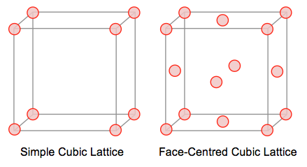
Given that each side of the lattice has a length of 1.07722, the volume of the unit cell will be $V=1.07722^3=1.25$

Since the density can be found using $\rho =\frac{N}{V}$, then in a simple cubic lattice containing one atom:

$\rho =\frac{1}{1.25}=0.8$

Next, a face-centered cubic lattice contains a total of 4 atoms. If the density of this unit cell is 1.2, the the length of one side can be found using:

$L={\left(\frac{4}{1.2}\right)}^{\frac{1}{3}}=1.49$

Figure 5: Simple Cubic and Face-Centred Cubic Lattices

Task 3

For the simple cubic lattice simulation, input file specified a total of 10 X 10 X 10 unit cells, giving a total of 1000 atoms as each simple cubic unit cell contains a single atom.

As mentioned above, a FCC lattice contains 4 atoms per unit cell. Therefore if a face-centred cubic lattice were defined rather a simple cubic lattice, the create_atoms command would produce a total of 4 x 1000 = 4000 atoms.

Task 4

Using the LAMMPS manual, the following commands could be better understood:

Mass 1 1.0

There is only one type of atom in the simulation, all with a mass of one.

Pair_style lj/cut 3.0

The Lennard-Jones potential between a pair of atoms will be calculated. However, due to the use of a global cutoff argument, the potential cannot be found if the inter-atomic distance between the two atoms is greater than 3 units. The cut-off value can be smaller or larger than the dimensions of the simulation box. This command neglects the contribution of Coulombic interactions.

Pair_coeff * * 1.0 1.0

This command specifies the force field coefficient of 1.0 units for the interacting atoms, giving a situation under which the above global cutoff value can be overridden. This changes the pair_style setting by resetting cutoffs for all atom type pairs. Here, the two asterisk signify that this applies for all pairs of atoms within the lattice.

NJ: Which coefficients?

Task 5

Since both $X_i(0)$ and $V_i(0)$ are specified, the velocity-Verlet algorithm must be adopted.

Task 6

### SPECIFY TIMESTEP ###
variable timestep equal 0.001
variable n_steps equal floor(100/${timestep})
variable n_steps equal floor(100/0.001)
timestep ${timestep}
timestep 0.001

### RUN SIMULATION ###
run ${n_steps}
run 100000

By writing the above code, instead of simply:

timestep 0.001
run 100000

It becomes easier to change the value of the timestep if desired. In the first version, once the first line reading 'variable timestep equal 0.001' has been changed, the rest of the code will be instantly updated. Conversely in the second version, you would have to re-read the entire code to find every mention of the previous value for the timestep for the calculation to work.

Specifically, the section quoted above ensures that no matter what the chosen timestep is, the same total time will always be simulated.

NJ: Good

Task 7

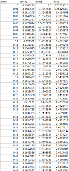
For the 0.001 timestep experiment, graphs showing energy, temperature and pressure vs. time were plotted. They all confirmed that the simulation reached equilibrium. All of the plots fluctuate about an average value and the gradient of the line of best fit is extremely small, of the order of 10^-5 and 10^-6. From figure 9, showing the raw data, it can be seen that equilibrium was reached after a time of 0.4 since all three of the parameters reach a value mirroring that of the y-intercept in their corresponding line of best fit equations (shown in figures 6, 7 and 8). Furthermore, three zoomed-in graphs of each parameter vs. time were created to confirm this.

Figure 6: Energy vs. Time at 0.001 Timestep

Figure 7: Temperature vs. Time at 0.001 Timestep

Figure 8: Pressure vs. Time at 0.001 Timestep

Figure 9: Raw Data and Zoomed E, T and P vs. Time at 0.001 Timestep

Next, an energy vs. time plot was made for all five different timestep experiments:

Figure 10: Energy vs. Time for all Five Timesteps

The longest timestep value of 0.015 shows an inconsistent result in that the simulation does not reach equilibrium and the energy is shown to gradually increase. The next four timestep values show much better results, with the two shortest 0.0025 and 0.001 fluctuating around the lowest energy value.

It can be concluded that a shorter timestep is necessary for simulations using the Lennard-Jones potential to establish an equilibrium with accurate results, as suggested in task 1. On the other hand, there comes a point where decreasing the timestep provides no additional benefits as a minimum energy is reached and a smaller timestep will only inhibit the simulation as the calculations take longer. In fact, the zoomed energy vs. time graph in figure 10 shows that a timestep of 0.0025 appears to fluctuate less than a timestep of 0.001 suggesting a more accurate average.

Overall, the 0.01 timestep is the largest to give acceptable results however 0.0025 is probably a better choice to obtain a set of more accurate results. On the other hand, the 0.015 timestep gives inaccurate results and an average is not reached.

NJ: Very nice explanation

Running Simulations Under Specific Conditions

Task 1

The temperatures chosen for the calculation are all above the critical temperature to ensure the simulation of a simple liquid and not a mixture of gas and liquid phases: T₁ = 1.5, T₂ = 2.0, T₃ = 2.5, T₄ = 4.0, T₅ = 6.0.

The pressures chosen are based on the simulations run previously: P₁ = 2.5, P₂ = 3.0

The timestep chosen was t = 0.0025

Task 2

In order to find the equation for $\gamma$ so that $T=\mathfrak{𝔗}$, we must start with:

$\frac{1}{2}\sum _i{m}_i{v}_i^2=\frac{3}{2}N{k}_{B}T$ $\frac{1}{2}\sum _i{m}_i{\left(\gamma v_i\right)}^2=\frac{{\gamma }^2}{2}\sum _i{m}_i{v}_i^2=\frac{3}{2}N{k}_B\mathfrak{𝔗}$

So:

$\frac{2{\gamma }^2}{2}*\frac{3}{2}N{k}_{B}T=\frac{3}{2}N{k}_B\mathfrak{𝔗}$ $\gamma =\sqrt{\frac{\mathfrak{𝔗}}{T}}$

Task 3

Looking at the command:

fix aves all ave/time 100 1000 100000 v_dens v_temp v_press v_dens2 v_temp2 v_press2

The fix command allows us to calculate the average for any defined thermodynamic property. The numbers that follow (Nevery, Nrepeat, and Nfreq arguments) specify on what timesteps the input values will be used in order to contributeto the average:

100 (Nevery) gives the number of timesteps that must pass before a sample value is taken to find an average. It must be a non-zero number.

1000 (Nrepeat) gives the number of samples that the final average comprises.

100,000 (Nfreq) and any of its multiples are the timesteps that generate the final averaged quantities. It must be a multiple of Nevery, and Nrepeat*Nevery cannot exceed Nfreq.

Hence there will be a sample taken every 100 timesteps, 1000 times until the data points reach a timestep of 100,000. Given that the timestep of the simulation was set to 0.0025, then 0.0025*100,000 = 250 time units will be simulated.

Task 4

The density vs. temperature graph for the ten simulations is shown below for P₁ = 2.5 and P₂ = 3. The error from both of these simulations was very small, shown by the tiny error bars in both the x and y directions. The two additional lines above the two experimental lines represent the value of the density at each pressure calculated using the ideal gas equation (k_B = 1 in reduced units):

$\rho =\frac{N}{V}=\frac{P}{k_{B}T}$

Figure 11: Density vs. Temperature for P = 2.5 and P = 3

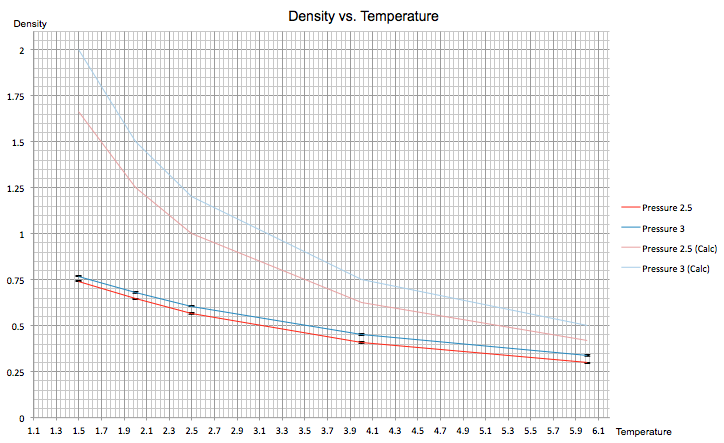
NJ: Consider drawing the graph without the grid, it might be clearer. Also, don't just join the points up for the ideal gas equation - if you have that few points, it's fine just to show the markers. Alternatively, you could fit a function to give a smooth line.

The density in both simulations is lower than the calculation. This can be explained by the fact that in the above equation we are looking at an ideal gas with no interactions between particles and therefore a potential energy of zero, whereas the simulations involve the calculation of the Lennard-Jones potential which, as discussed, considers the potential energy between two atoms. Hence there are attractive and repulsive terms between atoms that must be considered. As a result, the atoms in the simulation are located further from each other due to the Lennard-Jones potential between them and in turn this reduces the density.

Furthermore, the difference between the simulation and calculated density for P = 2.5 is smaller than at P = 3. Increasing pressure pushes particles closer together, so in an ideal gas the lack of interaction between the atoms mean they can move closer together quite easily. On the other hand, in the simulation the smaller interatomic distances lead to higher repulsive forces and hence the density at P = 3 is only slightly larger than at P = 2.5.

At higher temperatures, the difference between the simulated and calculated densities appears to converge. This occurs as a result of increased thermal motion; the atoms in the simulated liquid possess a higher kinetic energy which overrides repulsive forces between atoms, overall resulting in its behaviour becoming more ideal-like.

NJ: Good

Calculating Heat Capacities using Statistical Physics

Task 1

In statistical thermodynamics, the system is thought to fluctuate about an average equilibrium state. For example, if the temperature of the system is held 'constant' then the total energy must be fluctuating. The magnitude of the fluctuations in energy enable the heat capacity of the system to be determined and analysed. The equation for the heat capacity in the canonical ensemble is as follows:

$C_V=\frac{\partial E}{\partial T}=\frac{\mathrm{V}\mathrm{a}\mathrm{r}\left[E\right]}{k_B{T}^2}=N^2\frac{⟨E^2⟩-{⟨E⟩}^2}{k_B{T}^2}$

The numerator of the fraction contained in the equation above corresponds to the variance in the energy, ${\sigma }^2$ and N represents the total number of atoms in the system. The variance is the square of the standard deviation, $\sigma$, and is proportional to the fluctuations. In turn, the standard deviation is proportional to $\frac{1}{\sqrt{N}}$, telling us that a system containing a larger number of molecules will give smaller fluctuations and therefore a more accurate, better-defined average energy.

Shown below is a plot of $\frac{C_v}{V}$ as a function of temperature at two different densities, 0.2 and 0.8. The temperature ranges between 2.0 and 2.8. The graph follows the expected trend for an extensive property, where a higher density gives a higher value for $\frac{C_v}{V}$ since a system containing more particles requires more energy to increase the temperature of the system. The graph also shows a negative gradient in both cases despite the fact that with increasing temperature, the number of accessible energy levels is supposed to increased. This trend is perhaps arising from the fact that at higher temperatures the excited states are already occupied by electrons, making it less energetically favourable for further occupation to occur; overall, the transfer of heat to the system becomes more facile.

NJ: It's not just that there are more energy levels, it's that they are more closely spaced in energy. Therefore, to promote the system to a higher energy level (high temperature), less emergy is required. Be careful, these aren't electronic energy levels, so it's not electrons which are promoted. They're just "modes" of the system. It's not a specific idea, just an analogy.

Figure 12: Cv_V vs. Temperature

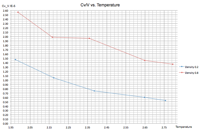
NJ: Again, I wouldn't connect the points by lines - this implies that there is a linear trend between the points, which there clearly isn't.

The following input script was used for the simulations (in this case, density = 0.2 and temperature = 2.0)

### DEFINE SIMULATION BOX GEOMETRY ###

variable d equal 0.2 

lattice sc ${d} 

region box block 0 15 0 15 0 15 

create_box 1 box 

create_atoms 1 box 


### DEFINE PHYSICAL PROPERTIES OF ATOMS ### 

mass 1 1.0 

pair_style lj/cut/opt 3.0 

pair_coeff 1 1 1.0 1.0 

neighbor 2.0 bin 


### SPECIFY THE REQUIRED THERMODYNAMIC STATE ### 

variable T equal 2.0 

variable timestep equal 0.0025 


### ASSIGN ATOMIC VELOCITIES ### 

velocity all create ${T} 12345 dist gaussian rot yes mom yes 


### SPECIFY ENSEMBLE ### 

timestep ${timestep} 

fix nve all nve 


### THERMODYNAMIC OUTPUT CONTROL ### 

thermo_style custom time etotal temp press 

thermo 10 


### RECORD TRAJECTORY ### 

dump traj all custom 1000 output-1 id x y z 


### SPECIFY TIMESTEP ### 


### RUN SIMULATION TO MELT CRYSTAL ### 

run 10000 unfix nve reset_timestep 0 


### BRING SYSTEM TO REQUIRED STATE ### 

variable tdamp equal ${timestep}*100 

fix nvt all nvt temp ${T} ${T} ${tdamp} 

run 10000 

reset_timestep 0 


### MEASURE SYSTEM STATE ### 

unfix nvt 

fix nve all nve 

thermo_style custom step etotal temp press density 

variable energy equal etotal 

variable energy2 equal etotal*etotal 

variable temp equal temp 

fix aves all ave/time 100 1000 100000 v_temp v_energy v_energy2 

run 100000 


variable avetemp equal f_aves[1] 

variable aveenergy equal f_aves[2] 

variable aveenergy2 equal f_aves[3] 

variable Cv_V equal (((atoms)^2)*(f_aves[3]-(f_aves[2])^2))/(vol*((f_aves[1])^2)) 


print "Cv_V ${Cv_V}" 

print "Temp ${avetemp}"

Structural Properties and the Radial Distribution Function

Task 1

The radial distribution function of a solid, liquid and gas in a Lennard-Jones system were found. The parameters used are as follows:

Gas $\rho =0.05$, $T=1.2$ in a simple cubic unit cell

Liquid $\rho =0.8$ and $T=1.2$ in a simple cubic unit cell

Solid $\rho =1.2$ and $T=1.2$ in a FCC unit cell

Figure 13: RDF of Solid, Liquid and Gas

The radial distribution function describes how density varies as a function of distance from a chosen particle in a system. Since it provides an average structure, it is a very good representation of a system; it doesn't just consider a single snapshot with 'instantaneous' disorder as it takes into the account the time. In all three cases above, the RDF only increases at an interatomic distance of about 0.9. Any smaller distances give an RDF of zero as at this distance the nuclei repel each other much too strongly to be placed so close together. The amplitude of the first peak for each curve is tallest in a solid and shortest in the gaseous system, as the particles are more densely packed in a solid relative to a gas.

NJ: The atoms repel, not the nuclei. There are no nuclei or electrons in the simulation, just point particles. But this is a good explanation otherwise.

The gas RDF shows a single peak at around r = 1. Since this single peak is broad we can reason that a gas has a large amount of disorder. There is neither short range nor long range order in the system.

The liquid RDF shows three peaks that decrease in amplitude with increasing separation. The peaks are less broad than in a gas and regularly spaced, suggesting a more ordered system. The presence of more than one peak indicates that the atoms pack around each other in 'shells', with the decreasing amplitude corresponding to the random Brownian motion of particles, leading to a decrease in order with an increase in separation. Due to the fact that the oscillations die away relatively quickly, it would suggest that only short range order is present in the system (specifically, between the first three nearest neighbours).

The solid RDF shows many sharp peaks that initially decrease in amplitude, and then a series of smaller fluctuating peaks through the remainder of the simulation. Since the peaks are sharp and narrow we know that the system is rigid and the atoms are strongly held in position and is therefore overall the most ordered system. The first three peaks can be related to specific lattice sites in the FCC unit cell upon which the simulation was based; A is the shortest distance and represents the tallest peak in the RDF whilst C is the largest distance and represents the third smaller peak. B represents the middle peak in the RDF, giving a lattice spacing of 1.475. Furthermore, the system appears to have both short and long range order due to the three large peaks (short) and the smaller fluctuating peaks (long).

NJ: Nice explanation. Is this the lattice spacing you would expect for this density? You could also use the values A and C to work out the lattice spacing, and then take an average - you can use your diagram to work out how far those distances are.

Figure 14: Lattice Sites Contributing to the RDF in FCC

The figure below shows the RDF integral vs distance for the solid system. The graph enables the coordination number of the three peaks to be determined since each point of inflection corresponds to a different coordination sphere. A central atom in a cluster of eight FCC unit cells will be neighbouring 12 atoms type A, so the first point of inflection corresponds to this point. Next, the central atom will be neighbouring 6 atoms of type B, corresponding to the second point of inflection given that 18-12 = 6. Finally, the central atom will be neighbouring 24 atoms of type C, and follows that this coordination sphere corresponds to the final point of inflection.

Figure 15: RDF integral of Solid

Dynamical Properties and the Diffusion Coefficient

Task 1

Using the liq.in file provided, three simulations were run for a gas, liquid and solid.

Task 2

The mean squared displacement, MSD, is a measure of the deviation in the distance between a moving particle and another reference particle. It can be defined by:

$MSD(\tau )=<r^2(\tau )>=<[r(t+\tau )-r(t){]}^2>$

The diffusion coefficient can be defined using this equation for the mean squared displacement:

$D=\frac{1}{6}\frac{\partial ⟨r^2\left(t\right)⟩}{\partial t}$

The plots of MSD vs. timestep of the three simulations mentioned previously are shown below.

Figure 15: MSD vs. Timestep Plots for a Solid, Liquid and Gas

The first two plots show the variation of the MSD with timestep when looking at a gaseous system. It can be seen that initially, the graph follows a parabolic relationship due to the fact that at the beginning of a simulation the gas atoms are placed at random, far from one-another. As a result there are fewer collisions between the atoms and interactions are small, overall resulting in each atom travelling at a constant velocity. At a constant velocity, the distance travelled per unit time is constant, so from the MSD equation above it follows that $MSD\propto t^2$. At a larger timestep, however, collisions become more frequent and the graph becomes linear to represent the Brownian motion of the gas particles. The second plot looks at the linear section in isolation, beginning on the 2000th timestep. This gave a more accurate value for the gradient and the value of $R^2$ increased from 0.98071 to 0.99833.

NJ: Very good

The third plot looks at a liquid system. It shows a strong linear relationship and a $R^2$ value of 0.9991. As discussed above this reflects the Brownian motion of the particles in the system, however since the particles in a liquid are much closer together than in a gas there is no preceding parabolic relationship.

Finally, the last plot for the solid crystal system shows a sharp increase to a MSD of about 0.02 and then fluctuates about that value for the rest of the simulation. This result occurs due to the fact that the atoms in the solid unit cell are strongly held in place; there is a limited amount of space available for them to move in and hence the value of the MSD has a small, finite value.

The value of the diffusion coefficient was calculated for each system:

Gas: $D=\frac{1}{6}*\frac{0.0364}{0.002}=3.03$

Liquid: $D=8.30*10^{-2}$

Solid: $D=5.83*10^{-7}$

As expected, the largest diffusion coefficient is calculated for the gaseous system as the less dense system has much more space in which the particles can move around each other. Conversely, the solid system is very rigid and closely packed, resulting in a very small diffusion coefficient.

The same plots were calculated for the same systems with 1 million atoms:

Figure 16: MSD vs. Timestep Plots for a Solid, Liquid and Gas (1 Million Atoms)

It can be seen that increasing the number of atoms didn't make any changes to the overall simulation. The only noteable change could be the smoothing in the fluctuations for the solid system. Hence it can be concluded that increasing the number of atoms by such a large amount is not necessary for these kinds of calculations.

The value of the diffusion coefficient for each system is almost identical to previously:

Gas: $D=\frac{1}{6}*\frac{0.0364}{0.002}=3.02$

Liquid: $D=8.30*10^{-2}$

Solid: $D=4.16*10^{-6}$

Task 3

From previously: $x=Acos(\omega t+\varphi )$ and so: $v=\frac{dx}{dt}=-A\omega sin(\omega t+\varphi )$

Given that $C(\tau )=\frac{\underset{-\mathrm{\infty }}{\overset{\mathrm{\infty }}{\int }}v(t)v(t+\tau )dt}{\underset{-\mathrm{\infty }}{\overset{\mathrm{\infty }}{\int }}{v}^2(t)dt}$

$C(\tau )=\frac{\underset{-\mathrm{\infty }}{\overset{\mathrm{\infty }}{\int }}-A\omega sin(\omega t+\varphi )\times -A\omega sin(\omega (t+\tau )+\varphi )dt}{\underset{-\mathrm{\infty }}{\overset{\mathrm{\infty }}{\int }}(-A\omega sin(\omega t+\varphi ){)}^{2}dt}$

$C(\tau )=\frac{\underset{-\mathrm{\infty }}{\overset{\mathrm{\infty }}{\int }}sin(\omega t+\varphi )\times sin(\omega (t+\tau )+\varphi )dt}{\underset{-\mathrm{\infty }}{\overset{\mathrm{\infty }}{\int }}si{n}^2(\omega t+\varphi )dt}$

$C(\tau )=\frac{\underset{-\mathrm{\infty }}{\overset{\mathrm{\infty }}{\int }}si{n}^2(\omega t+\varphi )cos(\omega \tau )dt}{\underset{-\mathrm{\infty }}{\overset{\mathrm{\infty }}{\int }}si{n}^2(\omega t+\varphi )dt}+\frac{\underset{-\mathrm{\infty }}{\overset{\mathrm{\infty }}{\int }}cos(\omega t+\varphi )sin(\omega \tau )sin(\omega t+\varphi )dt}{\underset{-\mathrm{\infty }}{\overset{\mathrm{\infty }}{\int }}si{n}^2(\omega t+\varphi )dt}$

Since $cos(\omega \tau )$ is a constant, it can be removed from the first integral and the two $si{n}^2(\omega t+\varphi )$ integrals cancel.

$C(\tau )=cos(\omega \tau )+sin(\omega \tau )\times \frac{\underset{-\mathrm{\infty }}{\overset{\mathrm{\infty }}{\int }}cos(\omega t+\varphi )sin(\omega t+\varphi )dt}{\underset{-\mathrm{\infty }}{\overset{\mathrm{\infty }}{\int }}si{n}^2(\omega t+\varphi )dt}$

Looking at the final fraction containing the two trigonometric integrals:

$\underset{-\mathrm{\infty }}{\overset{\mathrm{\infty }}{\int }}cos(\omega t+\varphi )sin(\omega t+\varphi )\to 0$. This is because $cos(\omega t+\varphi )sin(\omega t+\varphi )$ gives an odd function which is a combination of the even cosine function and the odd sine function, and therefore oscillates evenly about the x-axis. Hence as long as the limits of the integral are equal and opposite the area will be exactly zero.

$\underset{-\mathrm{\infty }}{\overset{\mathrm{\infty }}{\int }}si{n}^2(\omega t+\varphi )dt\to \mathrm{\infty }$. This is because a $si{n}^2(x)$ function always has positive y-values. Hence as the limits increase to infinity, so will the area.

So:

$C(\tau )=cos(\omega \tau )$

Next, on the same graph the harmonic oscillator VACF derived above and the VACF for the previous liquid and solid simulations were plotted between a timestep of 0 and 500.

Figure 17: VACF vs. Timestep Plots for a Lennard-Jones Solid and Liquid, and the Harmonic Oscillator

Firstly, at the minima observed for the two Lennard-Jones calculations there is a maximum difference between $v(t)$ and $v(t+\tau )$, reflecting the fact that the atoms are colliding and changing direction. The solid system shows a more negative value at this point as the interatomic forces are larger than they are in a liquid. Conversely, the points preceding these minima both give a maximum peak as at a timestep of zero, $v(t)$ and $v(t+\tau )$ have the same value.

For the solid VACF a series of further oscillations of decreasing amplitude reflect the very ordered lattice that the atoms occupy, because these atoms are strongly held in place they can oscillate back and forth but since the system is not perfect the oscillations will eventually die away. The liquid VACF shows just one minimum due to the fact that atoms only interact with their direct neighbours and no further.

NJ: Good. In fact, in the liquid, the minimum is the result of atoms colliding with their "solvent cage"

Both of these trends vary hugely from that of the VACF found for the harmonic oscillator, which shows a periodic function with no signs of decay. This is because the approximations in this system assume no energy loss as there is nothing for the harmonic oscillator to collide with. As a result, the velocity of the system does not get smaller.

Below is the VACF vs. timestep graph for a gas. This system exhibits no obvious oscillatory behaviour in the VACF throughout the simulation as the atoms are far apart and interact very weakly. This results in a much slower and gradual de-correlation in the velocity compared to the other more dense systems.

Figure 18: VACF vs. Timestep Plot for a Lennard-Jones Gas

Task 4

The trapezium rule was used to find the running integral under the VACF curves in the solid, liquid and gas simulations, shown in figure 19.

Since the diffusion coefficient can also be defined by:

$D=\frac{1}{3}\underset{0}{\overset{\mathrm{\infty }}{\int }}\mathrm{d}\tau ⟨\mathbf{v}\left(0\right)\cdot \mathbf{v}\left(\tau \right)⟩$

Then these graphs can be used to calculate $D$ by taking the point where the VACF integral reaches a plateau, hence the corresponding y-value provides the total integral of the velocity autocorrelation function.

Figure 19: VACF integral of Solid, Liquid and Gas

The value of the diffusion coefficient was calculated for each system:

Gas: $D=3.29$

Liquid: $D=9.78*10^{-2}$

Solid: $D=1.84*10^{-4}$

The same plots were calculated for the same systems with 1 million atoms:

Figure 20: VACF integral of Solid, Liquid and Gas (1 Million Atoms)

The value of the diffusion coefficient for each system is almost identical to previously:

Gas: $D=3.27$

Liquid: $D=9.01*10^{-2}$

Solid: $D=4.55*10^{-5}$

These calculated values follow the trend observed the diffusion coefficients in task 2 when using the mean squared displacement approach, with the gaseous system giving the largest value of $D$ and the solid system having the smallest. Once again, increasing the number of atoms doesn't have any significant effect on the value of the diffusion coefficient.

Despite both methods followed in calculating this coefficient provided results with similar values and approximately within the same order of magnitude, there are still a couple of discrepancies worth explaining, especially in the solid system. Given that this method used the trapezium rule to integrate the non-periodic VACF curves, errors are likely to have accumulated with time. However, the accuracy of the VACF method could be improved by either adopting a different method of integration or using a smaller trapezium. In this second option, however, it would be necessary to adopt a smaller timestep in the simulations. As discussed previously this is not always convenient as a shorter timestep takes longer to calculate.

NJ: Very good