Talk:Mod:ai513

Simulation of a Simple Liquid

---

Introduction

All data is attached in pdf format and is best viewed by clicking on it to open fully; some files have three pages.

---

Velocity Verlet Algorithm

Using the velocity verlet algorithm to model the behaviour of a classical harmonic oscillator, error was found between the solutions and the classical solutions. The classical solution was found according to the equation

$x=Acos(wt+\varphi )$

At a default timestep of 0.1, the function of error versus time was calculated as

$Error=0.0003t-0.0003$

File:Error for t=0.1

For the ensemble system to work correctly the total energy must not change by more than one percent over the whole calculation, and the value of timestep which reproduced this value was

$T=0.00939$

This is due to the fact that the system is in the NVE microcanonical ensemble and under Newton's laws of conservation of energy. For the system to perform accurately, this law must be obeyed as strictly as possible.

NJ: Good idea, but this is the error in the position, not the energy. NJ: Do you have any other plots from the harmonic oscillator?

---

Atomic Forces

For a single Lennard-Jones interaction,

$\varphi (r)=4ϵ\frac{{\sigma }^{(}12)}{r^{(}12)}-\frac{{\sigma }^{(}6)}{r^{(}6)}$

For the potential energy to be zero,

$r=\sigma ;$

which is equal to one half the internuclear distance. The force at this separation is

$F=24\frac{ϵ}{\sigma }$

The well depth (minimum potential energy) is as following:

$\varphi (eq)=-ϵ$ when $r(eq)=2^{\frac{1}{6}}\sigma$

Moreover, when σ = ε = 1.0:

$\int \varphi (r)dr=4(-\frac{1}{11r^{11}}+\frac{1}{5r^5})$

Therefore,

$\underset{2\sigma }{\overset{\mathrm{\infty }}{\int }}\varphi (r)dr=-2.48\times 10^{-3}$

$\underset{2.5\sigma }{\overset{\mathrm{\infty }}{\int }}\varphi (r)dr=-8.18\times 10^{-3}$

$\underset{3\sigma }{\overset{\mathrm{\infty }}{\int }}\varphi (r)dr=-3.29\times 10^{-3}$

These values show that from larger multiples of σ, the integrand becomes very small. The dominant, attractive part or the Lennard-Jones potential here quickly decreases with increasing separation. This is the basis of the lj-cutoff command described below. Any interactions with a separation greater than this cut-off are ignored as they do not contribute a significant to the overall forces in the system.

NJ: Nicely linked to the next section, but show your working.

---

Periodic Boundary Conditions

The number of molecules in 1mL of water: $1mL=1g$

$\frac{1}{18}=0.0555mol$

$0.0555\times Na=3.34\times 10^{22}molecules$

The volume of 10000 molecules of water:

$\frac{10000}{Na}=1.6\times 10^{-20}mol$

so

$1.6\times 10^{-20}\times 18=3\times 10^{-19}mL$

This is a reasonable number of atoms to work with, and illustrates why the volumes used in these simulations are therefore unrealistic and very small.

Considering a single atom in a cubic simulation box for one timestep, moving along the vector $(0.7,0.6,0.2)$, the atom will end up at position $(0.2,0.1,0.7)$ once the boundary conditions have been applied.

---

Reduced Units

For Argon,

$\sigma =0.34nm$ and $\frac{ϵ}{K}=120$ K

$r^{*}=3.2$ and $T^{*}=1.5$

$r=1.09\times 10^{-9}m$

$\varphi (eq)=-3.05\times 10^{-5}Kjmo{l}^{-1}$

NJ: This should be about 1 kJmol^-1. Not sure quite what has gone wrong without working.

$T=180K$

---

Equilibration

---

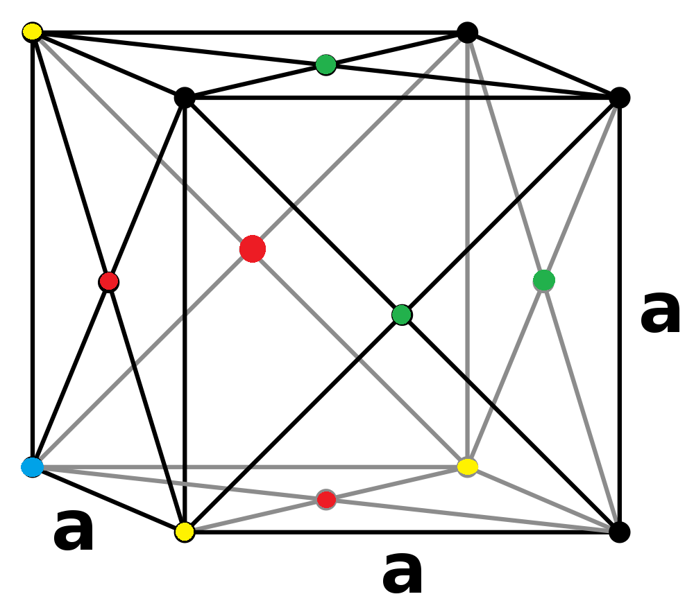
Creating the Simulation Box

When atoms are given random starting positions, and happen to be generated close together, the forces felt will be large and disproportionate to the average value in the actual system. This causes a problem as it will give unrealistic and incorrect acceleration and velocity values too.

In a simple cubic lattice of one lattice point (N=1), a lattice spacing of 1.07722 units corresponds to a number density of 0.8

$\frac{N}{V}=0.8$

$V=(1.07722{)}^3=1.25$

$\frac{N}{V}=0.7999\asymp 0.8$

When the lattice point number density of an FCC lattice (N=4) is 1.2 $r^{*}=1.49$

For a (10x10x10) simulation box of a FCC lattice 4000 atoms would be created.

---

Setting Atom Properties

mass 1 1.0

This command defines the variable mass, which atom type, and its actual mass.

pair_style lj/cut 3.0

This defines pairwise interactions, at a cut-off Lennard-Jones potential with no Coulomb, at a cut-off potential = 3.0σ.

pair_coeff * * 1.0 1.0

This defines a pairwise force field, for multiple atom pairs, where N=1. NJ: What do the numbers indicate?

The Velocity-Verlet algorithm would be used to specify X and V here.

Specifying the timestep is done as a variable ${timestep} so that the value can be varied easily, and different time steps can be used to optimise the system. For any timestep value, the number of time units is constant.

---

Checking Equilibration

File:2- E t P graphs.pdf

The simulation reaches equilibrium $E(av)=-3.184J$ at 0.38 time units.

$t=0.38\times 0.001=3.8\times 10^{-4}s$

File:3- E vs T.pdf

From this data, the optimal timestep chosen for further calculations was 0.0025. This is due to the fact that it is long enough that a sufficient amount of 'real' time is passed during simulation, but small enough that accuracy is maintained and thte system energy does not change as a function of timestep. The largest timestep of 0.015 allows for slow fluctuations in energy to be seen, know as explosions, and propagates atoms very close together causing augmented atomic collisions which produce a spike in F and E values. The total energy continually increases and doesn't reach equilibrium.

NJ: Okay, but how do you know 0.0025 is accurate enough? Why not 0.0075?

---

Calculating Heat Capacities

---

Temperature & Pressure Control

The system is changed from the micro canonical NVE to the isobaric-isothermal NpT ensemble for this section. From the previous section, the timestep used is

$t=0.0025$ and this simulation was run ten times at

$T*=1.8,2.1,2.4,2.7,3.0$

$P*=2.614,3.614$

From the equipartition theorem, the instantaneous temperature T can be calculated.

$Ek=\frac{3}{2}NKT$ and $Ek=\frac{1}{2}\sum m{v}^2$

This fluctuates through the simulation and the second equation must be changed to

$Ek=\frac{1}{2}\sum m(\gamma v{)}^2$

to give the target temperature, τ. The value of γ chosen so that T=τ is therefore:

$\gamma =\sqrt{(}(\frac{1}{2}m{v}^2)÷(\frac{3}{2}NKT))$

NJ: This can be simplified a bit further

---

Examining the Input Script

fix aves all ave/time 100 1000 100000

This refers to the frequency that the readings of average thermodynamic properties (stated after) are taken i.e. calculate the average values every 100000 time steps, using the 1000 input values before this step from every 100th piece of data

This means 1000 measurements will be sampled every 100000 time steps, over 1000 time units:

$t^{*}=100000\times 0.01=1000$

---

Plotting Equations of State

File:4- density graphs.pdf As pressure is increased in the simulation, the measured density increases.

At higher temperatures, the density decreases since the particles have more energy and can be repelled further.The simulated densities are lower than the theoretical values, due to the repulsive forces within a real system, resulting in a lower density. The discrepancy between theory and experiment decreases as temperature increases because the repulsive forces causing the differences are decreased relative to the now increased motion of the particles causing the density changes.

$PV=nRT$

$\frac{N}{V^{*}}=\frac{P^{*}}{T^{*}}$

The discrepancy between experimental and theoretical values increases as pressure is increased, because there are more atoms per unit volume and so the forces felt between atoms is larger as they are closer together.

NJ: You could provide a bit more detail here. What do you mean by "repulsive forces are decreased", for example?

---

Heat Capacities

---

Changing the Script for Density-Temperature Phases

The timestep used here is 0.0025, as any larger timestep results in energy fluctuations and a poor set of data.

File:Density 0.2 Temp 2.0 input script.log

File:5- Cv vs t.pdf

As temperature is increased, the heat capacity decreases. At higher pressures, heat capacity is higher. These results are unexpected of normal systems, however the liquid here functions like a classical harmonic oscillator. At higher temperatures the energy levels compress so that the system requires less thermal energy to change the temperature by a specific amount, i.e. the heat capacity decreases. At higher pressures the energy levels are also compressed, affecting the system as before.

NJ: Do you mean "at higher density"? What do you mean the liquid functions like a harmonic oscillator?

---

The Radial Distribution Function

---

Structural Properties

From the literature, phase transitions of LJ system the temperature and density of three states was found to be:

$Solid:T=1.0$ , $d=1.4$

$Liquid:T=1.0$ , $d=0.8$

$Gas:T=1.0$ , $d=0.05$

File:6- rdfs.pdf

These graphs show the difference between the probability of finding a particle at distance (r) from another particle in a solid, liquid and gas. All simulations were run with a timestep of 0.002. The graph of the solid is very noisy, where the regions of high and low probability show an ordered structure (fcc).

NJ: I know what you're trying to say, but noisy is the wrong word here. The peaks are very smooth. I'd say "there are many peaks, indicating a structured system">

The graph of the liquid is less erratic, and gas still further corresponding to the more continuous movement of particles in these states. This shows, as expected, that the particles become more and more diffuse as you move from solid to gas and the structure becomes more disordered and random. The integral of the RDF shows the cumulative coordination of the atoms, as r is increased, and the plateaus correlate to the area of one whole peak on the RDF.

NJ: The particles themselves don't become any more or less diffuse, but the system becomes less ordered.

In the solid state, the first three peaks correspond to the lattice sites of the 1st nearest neighbour , the second

and third
from the atom
being observed.

Base cube found from [1]

Peak #	r/σ	r (Å)
1	0.95	3.23
2	1.45	4.93
3	1.75	5.95

The lattice spacing is therefore 4.93Å as it's the second nearest neighbour. Alternatively, as the approximate trigonometric product of the 1st nearest neighbour:

NJ: How did you convert this to angstroms? It should be in reduced units. You should work out the distance that each neighbour you've indicated is located at, in terms of a, then get 3 estimates for a.

$a=\frac{\sqrt{2}}{2}\times 3.23\times 2=4.6$ Å

Or of the 3rd nearest neighbour:

$a=cos(\frac{45}{2})\times sin(\frac{45}{2})\times 2\times 5.95=4.2$ Å

The plateaus have values of 12 18 and 42, and therefore each peak has a coordination number of twelve, six and twenty-four respectively.

---

Diffusion Coefficient and Dynamical Properties

---

Mean Squared Displacement

The same values of temperature and density are used in these systems as before, to simulate a solid liquid and gas.

These graphs show how the mean squared displacement (the average measure of extent of random 3D motion within the system) varies with time, with a timestep of 0.002 and N=3375

$T=T^{*}\times 0.002$

The gradient of these graphs is equal to 6D therefore:

File:7- 3 state msd.pdf

State	Gradient	D
Solid	0.0057	9.5E-4
Liquid	0.4155	0.069
Gas	10.218	1.703

This process was repeated for one million atoms, and the graphs are shown below:

File:8- mill atom msd.pdf

State	Gradient	D
Solid	0.003	5E-4
Liquid	0.5132	0.086
Gas	12.54	2.090

These graphs show that solids have on average, the lowest diffusion coefficients, D. This is as expected, as D represents average motion of atoms in the system, and solid structures have the least motion. The gaseous systems have the largest diffusion coefficients, suggesting their atoms move around the most over a certain time-frame. This is also as expected. Finally, the plateau of the solid graphs is also in agreement with theory as the motion of particles should not change over time in a solid, as they do in a gas or liquid, and the motion of particles is constant and structured.

NJ: Why do you think the gas results are slightly curved?

---

Velocity Autocorrelation Function

Evaluating the normalized VACF for a 1D harmonic oscillator:

$Ct=\frac{\int V(t)V(\tau )dt}{\int V^{2}dt}$ and $\int V=X(t)$

As before, $x=Acos(\omega t+\varphi )$ and so;

Differentiating the function for position and subbing into the equaiton for Ct;

$Ct=\frac{\int -\omega A(sin(\omega t+\varphi )sin(\omega \tau +\varphi ))dt}{\int \omega A^{2}si{n}^2(\omega t+\varphi )dt}$

Rearranging gives

$Ct=\frac{-\omega A\int sin(\omega t+\varphi )\times [(sin(\omega t+\varphi )cos(\omega \tau )+cos(\omega t+\varphi )sin(\omega \tau ))]dt}{\int \omega A^{2}si{n}^2(\omega t+\varphi )dt}$

After some cancelling

$Ct=cos(\omega \tau )+sin(\omega \tau )\frac{\int sin(\omega t+\varphi )cos(\omega t+\varphi )dt}{\int si{n}^2(\omega t+\varphi )dt}$

Using rules of odd and even functions where sin is odd, cos is even, and the product of the two is odd:

$Ct=cos(\omega \tau )$

The following is a graph of velocity autocorrelations for a solid, liquid and the theoretical value, worked out from the solution above.

NJ: Be a bit tidier with your notation. The function you want, for example, is $C(\tau )$ not $Ct$

File:9- vacf s l theory.pdf

The minima in the VACFs for the solid shows periods of rapid negative motion that are the molecule's oscillations; the atoms vibrate showing periods of negative velocity at the end of each oscillation. The oscillations aren't of equal magnitude however, but decay in time because there are still destructive forces acting on the atoms to disrupt the perfection of the oscillatory motion. So what is seen is a function resembling damped harmonic motion.

NJ: Good effort. Be careful though, this isn't a molecule. What do you mean by destructive forces? The collisions between atoms cause the negative velocities.

The liquid behaves similarly to the solid, but now the atoms do not have fixed regular positions. Any oscillatory motion is destroyed by diffusion within the liquid. The VACF therefore shows one very damped oscillation and then decays to zero. This is expected, as it correlates to a collision between two atoms before they rebound from one another and diffuse away. The differences between the liquid and solid VACFs is due to the density of particles and particle motion. As established earlier, this liquid is less dense than the solid and so the liquid particles' motion is much more diffuse.

The theoretical harmonic oscillator VACF is different to the Lennard-Jones plots because in an actual system, the vibrational density of state does not go to infinity. In theory, the harmonic oscillator motion is smooth and uninterrupted by repulsive and attractive forces and the oscillatory cycle continues undisturbed to infinity.

NJ: The harmonic oscillator does experience attractive forces (but only to itself). There's nothing for it to collide with to lose correlation.

---

Finding the Diffusion Coefficient by Integration

Integrating the VACF graphs gives a value of $x=3D$

File:10- vacf and integ 3 state.pdf

State	Total Integral	D
Solid	0.000334	0.000
Liquid	0.247728	0.083
Gas	8.01832	2.673

This process was repeated for one million atoms, and the graphs are shown below:

File:11- mill atom vacf and integ.pdf

State	Total Integral	D
Solid	0.000137	0.000
Liquid	0.270274	0.090
Gas	9.805397	3.268

This data suggests that the vapour is more diffuse than the liquid, than the solid. This is as expected due to the lower density of vapour to liquid and solid, and its less ordered structure. Moreover, the dissusion coefficient for the solid is, in both simulations 0. This is because the atoms are in a fixed structure with very little motion. The high performance computer is very accurate, and so the largest source of error in these estimates of D from the VACF is the low number of atoms used (a constraint from the volume) and also fitting the integrals using the trapezium rule, as this is not a completely accurate way of finding the area of a graph.

NJ: How does this compare with your MSD results?