Talk:Mod:aed127

Third Year Simulation Experiment

Introduction

Molecular dynamics simulations examine how a set of atoms behave over a period of time, by using simplifications we can use these to simulate real systems and calculate thermodynamic properties of the system.

The Classical Particle Approximation

The Schrodinger equation can be used to describe the behaviour of a system, however, exact solutions are not possible and compromises must be made to reduce the complexity of the solutions so that they can be more easily computed. One such compromise is the classical particle approximation. It can be assumed that the atoms within the liquid act as a collection of N classical particles, therefore Newton’s second law can be used to give the following equation:

${\mathbf{F}}_i=m_i{\mathbf{a}}_i=m_i\frac{\mathrm{d}{\mathbf{v}}_i}{\mathrm{d}t}=m_i\frac{{\mathrm{d}}^2{\mathbf{x}}_i}{\mathrm{d}{t}^2}$

This equation allows both the positions and the velocities of the atoms to be calculated if it is known how the force changes with time.

Numerical Integration

Newton’s above equation can be integrated using a method called the Verlet algorithm, this is a numerical method that allows the positions of the atoms to be found at a time $t+\delta t$ upon specifying the initial conditions of the system. The Verlet algorithm requires the simulation to be discretised into timesteps of length $\delta t$ to allow us to solve the initial condition problem.

A problem with the Verlet algorithm is that it does not give the velocities of the atoms, so kinetic energy of the atoms cannot be calculated. A modified Velocity-Verlet algorithm is then used instead where it is assumed acceleration is only dependent on position, allowing velocities to be explicitly calculated.

TASK: Open the file HO.xls. In it, the velocity-Verlet algorithm is used to model the behaviour of a classical harmonic oscillator. Complete the three columns "ANALYTICAL", "ERROR", and "ENERGY": "ANALYTICAL" should contain the value of the classical solution for the position at time $t$, "ERROR" should contain the difference between "ANALYTICAL" and the velocity-Verlet solution (make sure you leave the half step rows blank!), and "ENERGY" should contain the total energy of the oscillator for the velocity-Verlet solution. Remember that the position of a classical harmonic oscillator is given by $x\left(t\right)=A\cos (\omega t+\varphi )$ (the values of $A$, $\omega$, and $\varphi$ are worked out for you in the sheet). Experiment with different values of the timestep. What sort of a timestep do you need to use to ensure that the total energy does not change by more than 1% over the course of your "simulation"? Why do you think it is important to monitor the total energy of a physical system when modelling its behaviour numerically? Why do you think the error in the position changes with time in the way that it does?

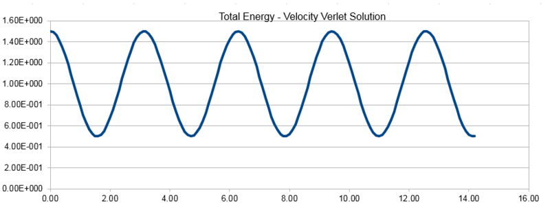
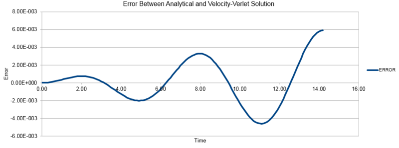
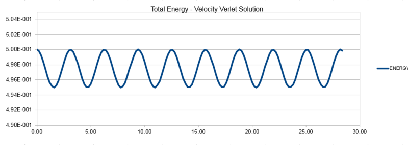
The three graphs below show the position calculated using the classical harmonic oscillator equation $A\cos (\omega \tau +\varphi )$, the energy as given by the Velocity-Verlet algorithm and the error between the position given by the two methods. The energy calculated here is the sum of the kinetic and potential energy at each given point.

NJ: Is this really the total energy? It's changing a lot!

Using a range of timesteps reveals that a timestep of lower than 0.2 must be used to keep the total energy from changing by less than 1% over the course of the simulation. This can be seen from the plot below, it was plotted using a 0.2 timestep and it can be seen that the total energy deviates by exactly 1% so we cannot use a larger timestep than this.

We see from the above error plot that the error between the classical and simulated solutions diverges over the course of the simulation, this is due to the chaotic nature of the particles in our simulation and their deviation from the ideal behaviours observed in the classical model. These deviations from the ideal behaviour compound upon one another as the simulation progresses, leading to the observed increase in divergence.

NJ: This simple example isn't a simulation of "particles", it's for a single harmonic oscillator (a single bead on a spring, if you like). This model isn't actually chaotic (although MD simulations of real systems are). Even though the function the magnitude of the errors grows over time, the absolute error still fluctuates (and is sometimes zero!).

When considering energy in our simulations, a conservation of energy would be expected when considering Newton's equations that the solutions arise from. In reality, we see an energy fluctuation in simulations, both in the short term and long term. The velocity-verlet algorithm shows good long term stability, and we monitor the total energy of the system to ensure there is no significant energy drift as this would lead to our simulations being unreliable for most purposes.

NJ: the energy fluctuations that you show wouldn't really be called long term — in fact, they are periodic at a single frequency.

Atomic Forces

We need to make simplifications again to determine the forces acting upon the atoms in our simulation, here classical physics tells us that the forces acting on our atoms are a result of the potential that they experience:

${\mathbf{F}}_i=-\frac{\mathrm{d}U\left({\mathbf{r}}^N\right)}{\mathrm{d}{\mathbf{r}}_i}$

The potential, U, that covers all the key interactions for the system can be modelled very well for simple liquids using the Lennard-Jones potential of the form:

$U\left({\mathbf{r}}^N\right)=\sum _i^N\sum _{i\ne j}^N\left\{4ϵ(\frac{{\sigma }^{12}}{r_{ij}^{12}}-\frac{{\sigma }^6}{r_{ij}^6})\right\}$

The Lennard-Jones potential gives an approximation of the interatomic potential between a pair of neutral species, it combines a short range repulsive term with a long range attractive term .

'TASK: For a single Lennard-Jones interaction, $\varphi \left(r\right)=4ϵ(\frac{{\sigma }^{12}}{r^{12}}-\frac{{\sigma }^6}{r^6})$, find the separation, $r_0$, at which the potential energy is zero. What is the force at this separation? Find the equilibrium separation, $r_{eq}$, and work out the well depth ($\varphi \left(r_{eq}\right)$). Evaluate the integrals $\underset{2\sigma }{\overset{\mathrm{\infty }}{\int }}\varphi \left(r\right)\mathrm{d}r$, $\underset{2.5\sigma }{\overset{\mathrm{\infty }}{\int }}\varphi \left(r\right)\mathrm{d}r$, and $\underset{3\sigma }{\overset{\mathrm{\infty }}{\int }}\varphi \left(r\right)\mathrm{d}r$ when $\sigma =ϵ=1.0$.

When potential energy is zero:

$0=4ϵ(\frac{{\sigma }^{12}}{r^{12}}-\frac{{\sigma }^6}{r^6})$

$0=\frac{{\sigma }^{12}}{r^{12}}-\frac{{\sigma }^6}{r^6}$

$\frac{{\sigma }^{12}}{{\sigma }^6}=\frac{r^{12}}{r^6}$

${\sigma }^6=r^6$

$\sigma =r$

The force at this separation is therefore equal to:

${\mathbf{F}}_i=-\frac{\mathrm{d}U\left({\mathbf{r}}^N\right)}{\mathrm{d}{\mathbf{r}}_i}$

${\mathbf{F}}_i=-4ϵ(\frac{-12{\sigma }^{12}}{r_0^{13}}-\frac{6{\sigma }^6}{r_0^7})$

Factoring in $\sigma =r$ gives force equal to

${\mathbf{F}}_i=-4ϵ(\frac{-12}{\sigma }+\frac{6}{\sigma })$

${\mathbf{F}}_i=\frac{24ϵ}{\sigma }$

The equilibrium separation of the potential is the minimum of the curve and therefore the value of r when the first derivative (force) is equal to zero:

$0=4ϵ(\frac{-12{\sigma }^{12}}{r_0^{13}}-\frac{6{\sigma }^6}{r_0^7})$

$2{\sigma }^6=r^6$

$2^{1/6}\sigma =r$

To find the well depth, i.e the value of $\varphi$ when at the equilibrium distance, we substitute the value of r_eq into the Lennard-Jones formula:

$\varphi =4ϵ(\frac{{\sigma }^{12}}{(2^{1/6}\sigma {)}^{12}}-\frac{{\sigma }^6}{(2^{1/6}\sigma {)}^6})$

Which ultimately gives:

$\varphi =-ϵ$

When the given integrals are evaluated with $\sigma =ϵ=1.0$

$\underset{2\sigma }{\overset{\mathrm{\infty }}{\int }}\varphi \left(r\right)\mathrm{d}r=-0.025$

$\underset{2.5\sigma }{\overset{\mathrm{\infty }}{\int }}\varphi \left(r\right)\mathrm{d}r=-8.17x10^{-3}$

$\underset{3\sigma }{\overset{\mathrm{\infty }}{\int }}\varphi \left(r\right)\mathrm{d}r=-3.29x10^{-3}$

NJ: Careful with rounding, the second one is $-0.8176\times 10^{-3}$. A little more working for the integration would have been better, but very good otherwise.

Periodic Boundary Conditions & Truncation

The simulations we run will only contain between 1000 and 10000 atoms, as it is too computationally demanding for us to simulate real volumes of liquid. In order for our simulations to approximate for real volumes of liquid we have to apply periodic boundary conditions. It is assumed that our atoms lie within a fixed box, which is repeated on all sides to avoid atoms at the box edge being exposed to a vacuum. If an atom passes over the edge of the box and into another box, it is instantaneously replaced by another atom entering from the other side to maintain a constant number of atoms.

TASK: Estimate the number of water molecules in 1ml of water under standard conditions. Estimate the volume of $10000$ water molecules under standard conditions.

1ml = 1g of water. M_r of water = 18g/mol.

Moles of water = 1/18

Number of water molecules = (1/18)*N_A = 3.35x10²² molecules

Number of moles in 10000 molecules = 10000/N_A

Mass = (10000N_A)*18gmol^-1 = 2.99x10^-19

Each 1g = 1ml = 1cm³ so, 2.99x10^-19/1 = 2.99x10^-19cm³

TASK: Consider an atom at position $(0.5,0.5,0.5)$ in a cubic simulation box which runs from $(0,0,0)$ to $(1,1,1)$. In a single timestep, it moves along the vector $(0.7,0.6,0.2)$. At what point does it end up, after the periodic boundary conditions have been applied?.

It ends up at point (0.2, 0.1, 0.7).

In order to avoid interactions between all atoms in our simulation the Lennard-Jones potential is often truncated to a set distance so those at such a distance that the interaction between them is almost zero are not included.

TASK: The Lennard-Jones parameters for argon are $\sigma =0.34\mathrm{n}\mathrm{m},ϵ=120/k_B\mathrm{K}$. If the LJ cutoff is $3.2\sigma$, what is it in real units? What is the well depth in $$\begin{gathered} {\mathrm{k}\mathrm{J} \\ \mathrm{m}\mathrm{o}\mathrm{l}}^{-1} \end{gathered}$$? What is the reduced temperature $T^{*}=1.5$ in real units?

The Lennard-Jones cutoff becomes = $3.2*0.34\mathrm{n}\mathrm{m}=1.09\mathrm{n}\mathrm{m}$ The well depth, $-ϵ$ is $=120*k_B*N_A/1000=0.10Kj/mol$ $T^{*}=1.5*120=180K$

NJ: good!

Equilibration

TASK: Why do you think giving atoms random starting coordinates causes problems in simulations? Hint: what happens if two atoms happen to be generated close together?

If atoms are generated too close together, their overlapping potentials causes a large force created between them, a high energy situation that would not happen in a real liquid. For this reason alone, giving atoms random starting positions is not a good starting point for a simulation as we can end up with the simulation 'exploding' and rather than reaching an equilibrium energy continually increasing in energy. To overcome this problem, we start our simulation with the atoms placed on the lattice points of a solid structure which is the melted to give a liquid.

NJ: the total energy might not continuously increase (at some point all of that potential energy will be converted to kinetic energy), but this is the right idea. The faster the atoms are moving, the shorter the timestep you need to use to accurately model the dynamics.

For the simulations run in this part of the experiment, a simple cubic lattice is used with a number density of 0.8, all specified by the command

lattice sc 0.8

In the output file the line

Lattice spacing in x,y,z = 1.07722 1.07722 1.07722

gives us the distance between lattice points to be 1.07722 in reduced units.

TASK: Satisfy yourself that this lattice spacing corresponds to a number density of lattice points of $0.8$. Consider instead a face-centred cubic lattice with a lattice point number density of 1.2. What is the side length of the cubic unit cell?

A simple cubic lattice has lattice points on the eight vertexes of a cube, therefore the distance between the lattice points is equal to the length of any edge of the cube. Knowing the cube edge lengths we can calculate the volume of the cube to be V = a³ = 1.07722³ = 1.25.

Each unit cell contains one atom and so the number density can be calculated to be 1/1.25 = 0.8

A face centered lattice has 4 atoms per unit cell and combined with the number density the volume can be calculated to be

density = number of atoms/volume

volume = number of atoms/density = 4/1.2 = 3.33

Side length = Volume^⅓ = 1.5

NJ: clear and simple explanation, well done.

TASK: Consider again the face-centred cubic lattice from the previous task. How many atoms would be created by the create_atoms command if you had defined that lattice instead?

As previously mentioned, we set periodic boundary conditions to simulate our atoms within a box of set dimensions. In the input script we define our box using the lines

region box block 0 10 0 10 0 10
create_box 1 box

Which in the output file, gives us a defined box:

Created orthogonal box = (0 0 0) to (10.7722 10.7722 10.7722)

This created box contains 1000 unit cells, which corresponds to 1000 atoms in our simulations using the simple cubic lattice. If the face centered cubic lattice, which contains 4 atoms per unit cell, 4000 atoms would be created.

NJ: Good.

TASK: Using the LAMMPS manual, find the purpose of the following commands in the input script:

mass 1 1.0
pair_style lj/cut 3.0
pair_coeff * * 1.0 1.0

The line mass 1 1.0 is a command of the general form mass I value, where I specifies the atom type, it can have any numerical value corresponding to pre set atom types or asterisks can be used as a wildcard term for multiple atom types, and 'value' is replaced by the desired mass of the atoms.

pair_style lj/cut 3.0 specifies the formulas used by LAMMPS to model interactions between atoms. For this example, lj/cut refers to the Lennard-Jones model with a cutoff at 3.0 distance units.

Lastly, pair_coeff * * 1.0 1.0 provides the force coefficients for intermolecular interactions. The asterisks work in the same way as previously mentioned, in this case * * sets the coefficients for all atom types in the simulation and gives them values of 1.0 and 1.0.

NJ: Which parameter is which? TASK: Given that we are specifying ${\mathbf{x}}_i\left(0\right)$ and ${\mathbf{v}}_i\left(0\right)$, which integration algorithm are we going to use?

The verlet method only specifies the position in it's initial conditions, if we also wish to specify the initial velocity we can use the Velocity-Verlet algorithm.

NJ: Yes. In fact, LAMMPS always uses velocity-Verlet, and if we don't specify initial velocities it sets them all to 0. TASK: Look at the lines below.

### SPECIFY TIMESTEP ###
variable timestep equal 0.001
variable n_steps equal floor(100/${timestep})
variable n_steps equal floor(100/0.001)
timestep ${timestep}
timestep 0.001

### RUN SIMULATION ###
run ${n_steps}
run 100000

The second line (starting "variable timestep...") tells LAMMPS that if it encounters the text ${timestep} on a subsequent line, it should replace it by the value given. In this case, the value ${timestep} is always replaced by 0.001. In light of this, what do you think the purpose of these lines is? Why not just write:

timestep 0.001
run 100000

Assigning the timestep a value in this way allows us to control the value of the timestep throughout the input script, as the value is often repeated in other parts of the script with reference to other commands, writing out a full definition for the timestep rather than just using the two lines ensures timestep is defined and constant over the whole simulation.

NJ: Not quite. By doing it this way, we make sure that we run for 100 time units, no matter what the timestep is. That's important for comparing the energies in the next section.

TASK: make plots of the energy, temperature, and pressure, against time for the 0.001 timestep experiment (attach a picture to your report). Does the simulation reach equilibrium? How long does this take? When you have done this, make a single plot which shows the energy versus time for all of the timesteps (again, attach a picture to your report). Choosing a timestep is a balancing act: the shorter the timestep, the more accurately the results of your simulation will reflect the physical reality; short timesteps, however, mean that the same number of simulation steps cover a shorter amount of actual time, and this is very unhelpful if the process you want to study requires observation over a long time. Of the five timesteps that you used, which is the largest to give acceptable results? Which one of the five is a particularly bad choice? Why?

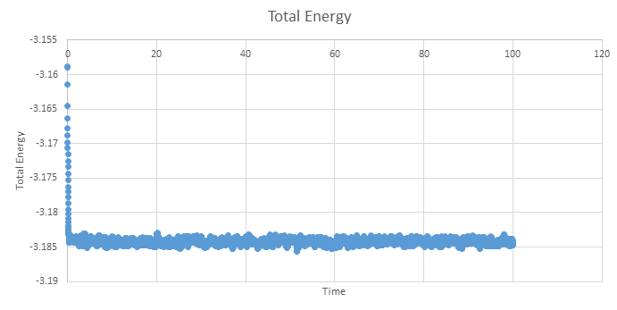
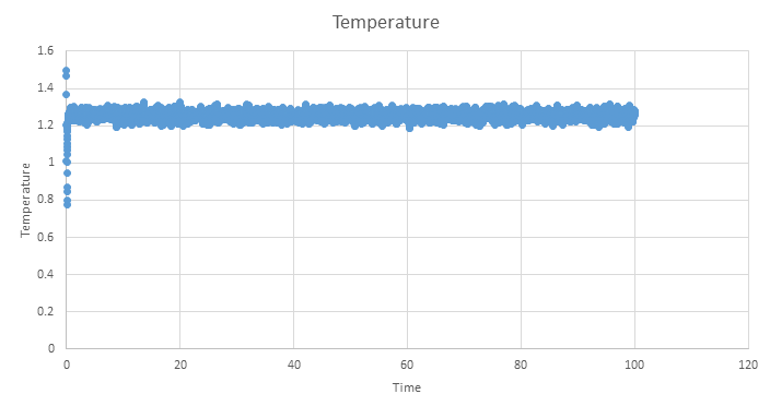
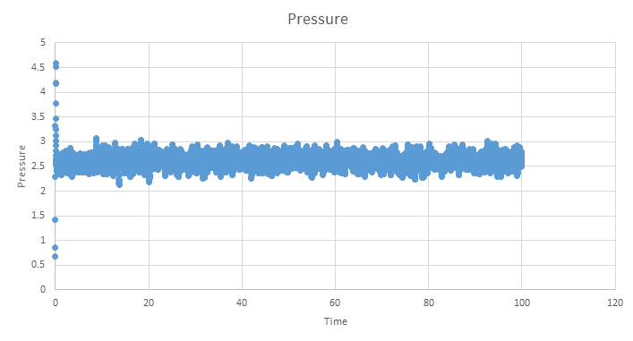
Below are the plots of energy, temperature and pressure against time for the 0.001 timestep simulation, units are reduced and therefore dimentionless. These plots show that an equilibrium is reached, however we see short range fluctuations about the equilibrium. As mentioned earlier, these are a seen when using the velocity verlet algorithm as it does not have great short range stability.

NJ: it's true that Verlet does cause fluctuations in the energy (even in the "NVE" ensemble). That's a combination of numerical error by the computer, and problems introduced by discretisation. Remember though, that not all properties are meant to be totally constant. In the NVE ensemble, it is perfectly normal for pressure to fluctuate. How do you know that equilibrium is reached?

NJ: this might be clearer if displayed with a thin line, instead of with points.

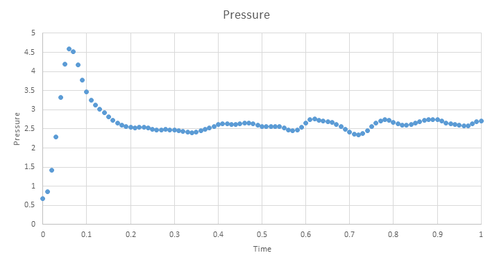
Zooming in on the plot shows that the simulation only needs a short amount of time to reach a equilibrium and is reached by ~0.5 time units.

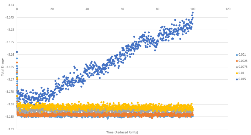
Below is a plot that shows the same simulation run five times but with varying time steps between 0.001 and 0.015. As can be seen, the 0.015 timestep is a particularly bad choice of timestep as rather than the simulation reaching an equilibrium as is the case with all the other timesteps, we see the simulation continually increasing in energy. It is no coincidence that 0.015 is also the largest timestep used, using a timestep that is too large can cause the simulation to become unstable causing the 'exploding' behaviour observed. This 'exploding' happens when too large a timestep causes two atoms to be moved to points where they have nearly overlapping or overlapping potentials, causing a very large force that drives the atoms apart.

Timesteps 0.001 to 0.01 show the expected behviour of settling down to a constant value (with short range fluctuations around the mean value), however perhaps not expected is the slight increase in the total energy with increasing timestep. This trend can be understood in similar principles to the 0.015 example, a longer timestep means the atoms in the simulation are propagated more than in shorter timestep simulations. This leads to an increased probablility that atoms will move into a more energetically unfavourable state in any given timestep than in a shorter timestep case.

NJ: What do you think the largest timestep that you can reasonably use is? Again, this graph might be a little clearer if you used thin lines rather than points.

Simulations Under Specific Conditions

Up until this point, simulations had been described by the microcannonical ensemble, nVE, in which the number of atoms, volume and total energy are held constant. In this section of the experiment, the conditions are changed so simulations are run under the npT ensemble, this allows the equation of state for the simulation to be plotted, as will be done below.

In order to control the temperature of the system, the instanteous temperature, T, is calculated at the end of each timestep and used to determine the value of a constant $\gamma$. This constant is then used to multiply each velocity to bring the temperature T to the target temperature, $\mathfrak{𝔗}$.

TASK: We need to choose $\gamma$ so that the temperature is correct $T=\mathfrak{𝔗}$ if we multiply every velocity $\gamma$. We can write two equations:

$\frac{1}{2}\sum _i{m}_i{v}_i^2=\frac{3}{2}N{k}_{B}T$

$\frac{1}{2}\sum _i{m}_i{\left(\gamma v_i\right)}^2=\frac{3}{2}N{k}_B\mathfrak{𝔗}$

Solve these to determine $\gamma$.

In order to solve for $\gamma$, the second of the two equations can be divided by the first giving:

${\gamma }^2=\frac{T}{\mathfrak{𝔗}}$

and therefore

$\gamma ={\left(\frac{T}{\mathfrak{𝔗}}\right)}^{\frac{1}{2}}$

NJ: Good — just a little more working would have been better (a note to the effect that gamma can be taken outside the sum, for example).

In the input file, lines are specified that control which thermodynamic properties are recorded. In order to be able to caluclate the equation of state we need to know the average temperature, density and pressure along with the standard errors in each value. These lines are as follows:

### MEASURE SYSTEM STATE ###
thermo_style custom step etotal temp press density
variable dens equal density
variable dens2 equal density*density
variable temp equal temp
variable temp2 equal temp*temp
variable press equal press
variable press2 equal press*press
fix aves all ave/time 100 1000 100000 v_dens v_temp v_press v_dens2 v_temp2 v_press2
run 100000

TASK: Use the manual page to find out the importance of the three numbers 100 1000 100000. How often will values of the temperature, etc., be sampled for the average? How many measurements contribute to the average? Looking to the following line, how much time will you simulate?

The three values on the final input line shown above correspond to the general input commands Nevery Nrepeat Nfreq respectivley. Nevery tells the programme to use the input values every this number of timesteps, 100 in this case, i.e the values of pressure, temperature, etc. will be sampled every 100 timesteps. Nrepeat specifies the number of times to use the input values for calculating averages and Nfreq is the number of timesteps in between calculating averages.

Overall we can understand this as a taking a sample every 100 steps 1000 times until 100000 timesteps have passed. As 100*1000 = 100000 we get an output of only one average value.

NJ: How much time is simulated?

TASK: When your simulations have finished, download the log files as before. At the end of the log file, LAMMPS will output the values and errors for the pressure, temperature, and density $\left(\frac{N}{V}\right)$. Use software of your choice to plot the density as a function of temperature for both of the pressures that you simulated. Your graph(s) should include error bars in both the x and y directions. You should also include a line corresponding to the density predicted by the ideal gas law at that pressure. Is your simulated density lower or higher? Justify this. Does the discrepancy increase or decrease with pressure?

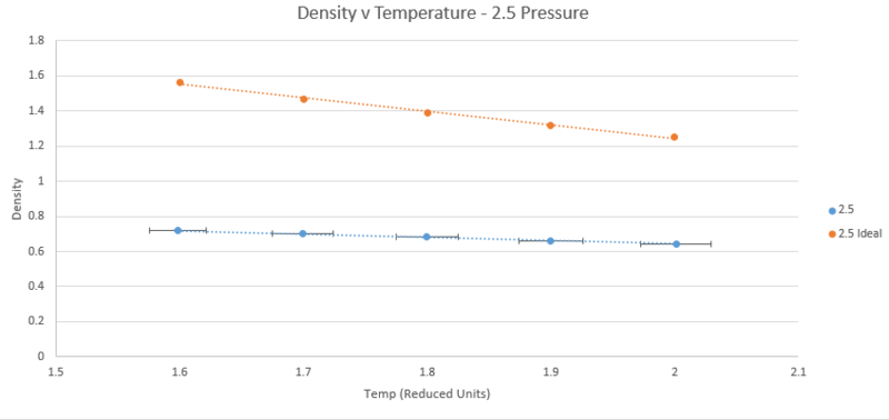
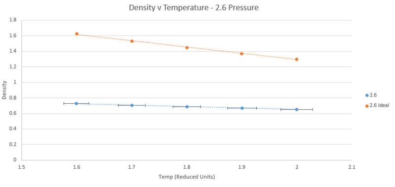
The plots below show five plotted temperatures 1.6, 1.7, 1.8, 1.9, and 2.0 at two different pressures 2.5 and 2.6 under the npT ensemble, as well as the density described by the ideal gas law n/v = P/T (Kb is simply one in reduced units). Each plot of the simulated data has error bars in both directions taken from the standard error printed in the output files. On the scale shown, however, the vertical error is too small to be shown.

As shown by both plots, the simulated density is always lower than that predicted by the ideal gas law. The ideal gas law operates under the assumption that there are no interactions between atoms. At high temperatures and low pressure this holds true as kinetic energy dominates or molecules are so far apart that interactions are negligible. It therefore follows that when temperature is increased or pressure decreased in the simulation, the discrepancy between the simulation and the ideal gas law diminishes. This can be clearly seen on the graphs for the temperature case but not for pressure. Examination of the plots of both pressures at temperature 2 units shows the difference between the simulated and ideal cases is 0.60547501 at 2.5 pressure and 0.647793557 at 2.6 pressure, confirming that the discrepancy decreases with decreasing pressure.

NJ: Very nice — unluckily, you picked two pressures that are very close together, so there's not much difference. Obviously, there's no way to know how big a difference 0.1 pressure units is without doing the conversion.

Calculating Heat Capacities

The heat capacity of the system is related to the fluctuation of the system from the average value and can be described by the equation:

$C_V=\frac{\partial E}{\partial T}=\frac{\mathrm{V}\mathrm{a}\mathrm{r}\left[E\right]}{k_B{T}^2}=N^2\frac{⟨E^2⟩-{⟨E⟩}^2}{k_B{T}^2}$

In order to run a simulation that will allow us to calculate the heat capacity of the system, modifications to the input scripts previously used must be made. A simulation in which a lattice crystal is melted and reaches equilibrium is used as before, except it now runs under the NVT ensemble. In order to fix to this ensemble, a command is introduced to fix the density of the lattice. Once the system is in equilibrium, the thermostat is switched off. Both the average energy and the average energy squared are printed to the output to allow the heat capacity to be calculated.

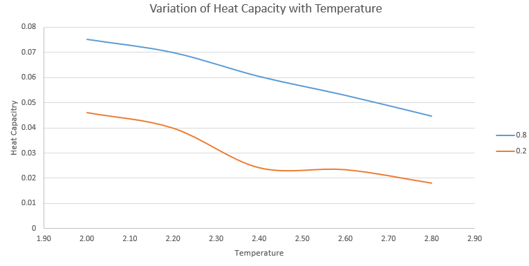
The simulation was run at two densities, 0.2 and 0.8 and 5 temperatures 2.0, 2.2, 2.4, 2.6, and 2.8 to give ten values of the heat capacity which are plotted on the graph below. The heat capacities are given per unit volume to allow a comparison to be made between the two densities.

An example input script can be found here: 2.0, 0.2 Input

The plot above shows constant volume heat capacity at the two densities as you can see , the heat capacity at larger density is greater. This is due to a higher number of atoms per unit volume at density 0.8 than the 0.2 and as the heat capacity is an extensive property with respect to the number of molecules, we see a higher heat capacity when more atoms are present.

NJ: You can argue that you've got more interactions in the denser system, so more degrees of freedom that you can pump energy into.

NJ: What about the trend with temperature?

NJ: What about the kink? Do you think that is physical, or an artefact of the simulation?

TASK: As in the last section, you need to run simulations at ten phase points. In this section, we will be in density-temperature $({\rho }^{*},T^{*})$ phase space, rather than pressure-temperature phase space. The two densities required at $0.2$ and $0.8$, and the temperature range is $2.0,2.2,2.4,2.6,2.8$. Plot $C_V$ as a function of temperature for both of your densities (on the same graph). Is the trend the one you would expect? Attach an example of one of your input scripts to your report.

Structural Properties and the Radial Distribution Function

In this section of the experiment, we plot the radial distribution function to explore the structure of our simulated systems. The radial distribution function, denoted $g(r)$ describes the density of the system as a function of the distance from a given reference point. It can also be explained as a measure of the probability of finding an atom at a distance $r$ from the reference point, relative to an ideal gas.

TASK: perform simulations of the Lennard-Jones system in the three phases. When each is complete, download the trajectory and calculate $g(r)$ and $\int g(r)\mathrm{d}r$. Plot the RDFs for the three systems on the same axes, and attach a copy to your report. Discuss qualitatively the differences between the three RDFs, and what this tells you about the structure of the system in each phase. In the solid case, illustrate which lattice sites the first three peaks correspond to. What is the lattice spacing? What is the coordination number for each of the first three peaks?

The program VMD is used to produce a plot of both $g(r)$ and its running integral $Int(g(r))$ from simulations of the Lennard-Jones system in the solid, liquid and gas phases. The density and temperature of the input script were modified to simulate for each phase and a simple cubic lattice was used for liquid and vapour phases, with face centered cubic used for the solid phase.

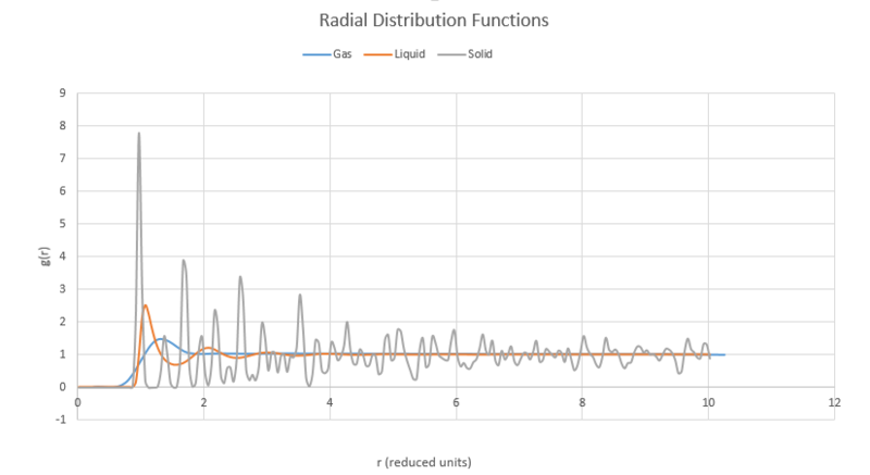
Below are all three radial distribution functions shown on the same axes.

All plots start at very low density, as there is very little probability of finding another atom at these short distances as it is very energetically unfavourable to have another atom so close. All plots then rise to an initial peak corresponding to its nearest neighbour. For the solid, this is understandably fairly close to the initial position as the atoms are fixed and ordered in the lattice, each subsequent peak in the solid is its subsequent nearest neighbour found at regular intervals, inferring the structured nature of the solid crystal.

The gas plot shows only one peak before falling off to a flat value. This infers that the gas molecules are likely to have particles relatively close and then no long range regular spacing. For the liquid case, we see an intermediate between the other two cases with two peaks before levelling off. This reflects the nature of the liquid being somewhere between that of a solid, with some regular order but still much more constrained than the gas.

NJ: The typical nomenclature is that crystalline solids have "long range order", liquids have short range order but no long range order, and gases are disordered.

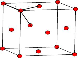
The identity of the first three lattice points in the solid case can be designated by looking at the structure of the face centered cubic lattice:

From this diagram the three nearest neighbours, a, b and c, respectively, can be seen. These three nearest neighbours are the first three peaks in the RDF plot.

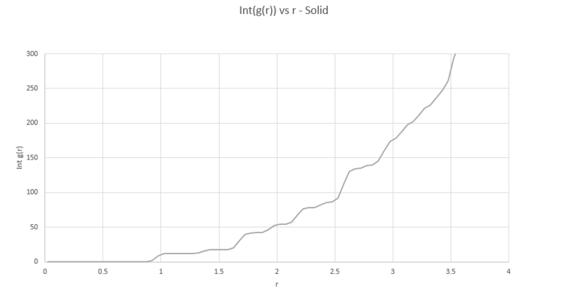
We can also use the plots of RDF for the solid to determine the coordination number of these three nearest neighbours. In order to do this we must find the points at which the three peaks collapse, which correspond to the points r= 1.05, 1.45 and 1.75

We then cross reference these r values with the running integral (plotted above) which gives values of 12, 18 then 42. We need to subtract the areas of the preceding peaks for the second and third coordinations leaving us with coordinations of 12, 6 and 24 for the three neighbours. As the second nearest neighbour is along the lattice edge, the distance of this atom also corresponds to the lattice spacing, giving a spacing value to be: 1.45

NJ: Very good - how did you judge where to measure the start of the plateau for the second neighbour? It might be easier to measure the position of the peak instead. You could also have used the positions of subsequent peaks to improve your estimate.

Dynamical Properties and the Diffusion Coefficient

The atoms in our simulations do not stay in a fixed position throughout the simulation, instead they are constantly moving on a 'random walk' where each step taken is in a direction unrelated to the step taken before it. The mean square of the displacement made on this walk $<r^2>$ can allow us to calculate the diffusion coefficient using the below equation:

NJ: this is an approximation to how atoms move!

$D=\frac{1}{6}\frac{\partial ⟨r^2\left(t\right)⟩}{\partial t}$

TASK: make a plot for each of your simulations (solid, liquid, and gas), showing the mean squared displacement (the "total" MSD) as a function of timestep. Are these as you would expect? Estimate $D$ in each case. Be careful with the units! Repeat this procedure for the MSD data that you were given from the one million atom simulations.

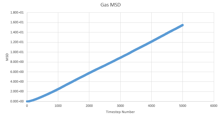
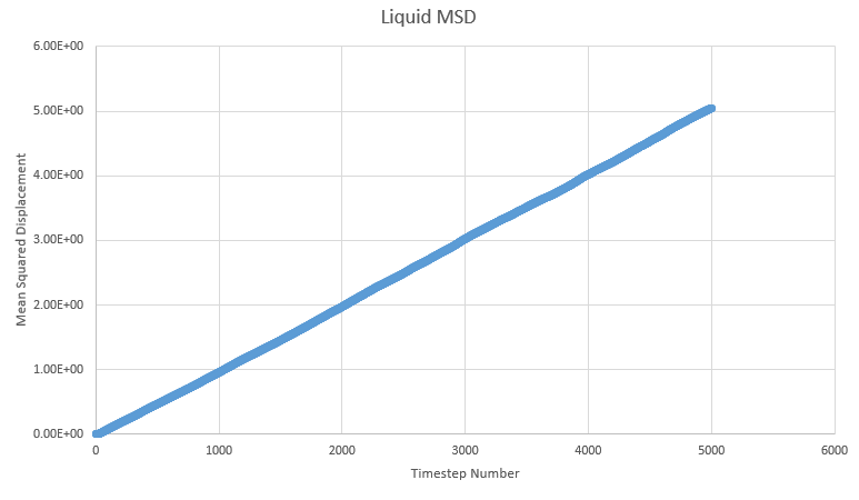
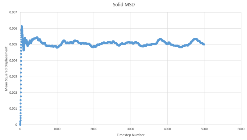
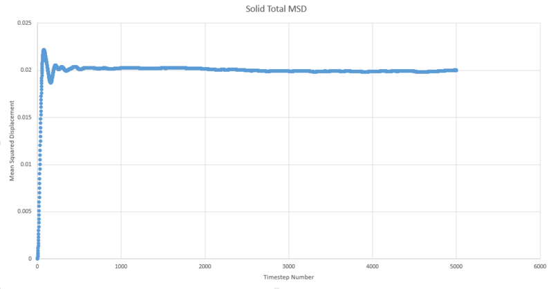
One of the outputs for the simulations previously run for the radial distribution function provides us with the mean squared displacement each of which are plotted below as a function of timestep.

In order to estimate D from each plot, the gradient of each plot was taken once linearity had been judged to have been reached and then multiplied by \frac{1}{6} to give values of 51.7, 0.000171 and 4.68x10^-10 for gas, liquid and solid respectivley.

We expect to see a very large diffusion coefficient for gas relative to the others due to the fact the molecules in the gas are far apart and so freely able to move around, liquids are freely able to move around each other within the bulk of the liquid but are not completely separated from the other molecules, reflected in the high, but lower than gas diffusion constant. The solid shows a very small diffusion coefficient due to the very small range of movement available to it in its crystal lattice structure. Each atom in the solid is tightly packed into a regular structure and only really shows vibration.

We expect to see a linear plot of mean squared displacement as the atom should be constantly moving at a regular pace, thus always increasing the MSD at a linear pace. We observe an almost perfect linear plot for the liquid and gas cases, with the gas only showing a small curve at the beginning of the plot. This curve is seen because the gas atoms take a little while to reach an energy equilibrium and it is not until this is reached that we see a linear plot.

The shape observed for the solid lot is due to the aforementioned restricted motion of the atoms in the solid lattice.

Shown below are the plots of mean squared displacement against time plotted for the one million atom simulation:

As can be seen, they display very similar shapes to the MSDs plotted before with fewer atoms. The main difference that can be seen is the million atom plots appear to be smoothed out in comparison to the plots with fewer atoms. The values of D calculated from the million atom plots vary compared to the previously calculated values at 0.005081494,0.000176124, -1.75837x10^-08 for vapour, liquid and solid respectivley. However, we do see the same trend as before and a very similar value for the liquid MSD.

NJ: does the value for the solid seem physical to you? Does it make sense that the results are smoother when there are more atoms?

NJ: plot the fitted lines, and show the equations.

NJ: It would be good to have a table comparing the D values for the three phases from both sets of simulations. Your D values seems very small, I think they might still be in "timestep" units rather than "time" units.

Velocity Auto Correlation Function (VACF)

$C\left(\tau \right)=⟨\mathbf{v}\left(t\right)\cdot \mathbf{v}(t+\tau )⟩$

The VACF gives us an alternate method to calculate the diffusion constant. This function tells us how different the velocity is between time $t$ and $t+\tau$. We can calculate the diffusion constant by simply integrating this function:

$D=\frac{1}{3}\underset{0}{\overset{\mathrm{\infty }}{\int }}\mathrm{d}\tau ⟨\mathbf{v}\left(0\right)\cdot \mathbf{v}\left(\tau \right)⟩$

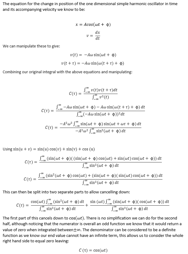
TASK: In the theoretical section at the beginning, the equation for the evolution of the position of a 1D harmonic oscillator as a function of time was given. Using this, evaluate the normalised velocity autocorrelation function for a 1D harmonic oscillator (it is analytic!):

$C\left(\tau \right)=\frac{\underset{-\mathrm{\infty }}{\overset{\mathrm{\infty }}{\int }}v\left(t\right)v(t+\tau )\mathrm{d}t}{\underset{-\mathrm{\infty }}{\overset{\mathrm{\infty }}{\int }}{v}^2\left(t\right)\mathrm{d}t}$

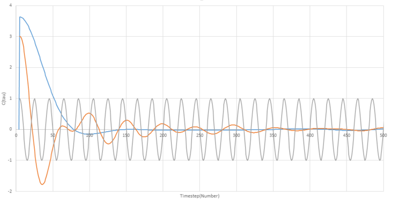
Be sure to show your working in your writeup. On the same graph, with x range 0 to 500, plot $C\left(\tau \right)$ with $\omega =1/2\pi$ and the VACFs from your liquid and solid simulations. What do the minima in the VACFs for the liquid and solid system represent? Discuss the origin of the differences between the liquid and solid VACFs. The harmonic oscillator VACF is very different to the Lennard Jones solid and liquid. Why is this? Attach a copy of your plot to your writeup.

NJ: you stopped distinguishing between $t$ and $\tau$ at some point in this derivation. Remember that you *can't* take $t$ out of the integral, only $\tau$. Strictly speaking, the result you've derived says that C is a constant.

Using this equation and a value of ω to be 1/2π the harmonic oscillator was also plotted alongside the VACF for a liquid and a solid. On the plot below, the VACF for the solid is shown in orange, the liquid is shown in blue and the harmonic oscillator in grey.

For both the liquid and solid plots the shape of the curve, the shape can be understood by talking about what is happening to the particle over time timescale. Initially, both plots show a rapid drop, this is due to the velocity changing due to collisions with other particles in the medium. In the liquid model, a small negative minimum is reached before the plot settles at zero, confirming the long range uncorrelation of the velocity. The solid plot also shows some oscillation about zero before also settling to a zero value.

NJ: the solid doesn't quite get there in your example, but it will do eventually.

The minima in the plots are point at which the velocity shows a negative correlation with the initial velocity and can be attributed to so called 'backscattering' regions where the particles can be imagined to be moving back and forth within a temporary block of surrounding particles. Another way of looking at negative regions on the plot is that they describe collisions that produce large angle deflections of near 180°

NJ: this is correct. In fact, any deflection beyond 90 degrees will give negative correlation. In more chemical terms, it's often attributed to molecules colliding with their "solvent cage".

The differences between the plots of solid and liquid VACFs arise from the degree of constraint of the atoms involved, the molecules in the liquid are much more 'free' to self-diffuse and move around in the fluid than particles in the solid, which are constrained by the lattice structure.

NJ: alternatively, a liquid can move further before it collides with another atom.

For this reason we see the liquid VACF decay to zero much faster than the corresponding solid plot, as it is collisions and self diffusion that result in the eventual non-correlation of the velocity to the orignal value. The solid plot retains some correlation at longer time periods, and takes a shape resembling that of a damped simple harmonic oscillator, to explain why this is, we must examine the origins of the harmonic plot.

NJ: it's a little more complex than that — you can compare it to the simple HO plot between 50 and 100 time units to see that the solid VACF differs by more than a multiplicative factor.

The harmonic oscillator is completely unaffected by external forces and as such does not undergo collisions of any kind or self diffuse. For this reason, we see the harmonic oscillator describe a constant periodic function that remains correlated to it's initial velocity due to a lack of external interference. Revisiting this solid plot, we can understand that it decays to zero much slower than the liquid due to not being free to collide to the extent that the liquid is, and only suffering smaller external forces when vibrating in the solid and feeling intermolecular forces from surrounding atoms.

NJ: very good.

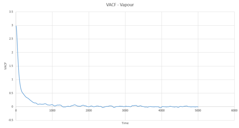
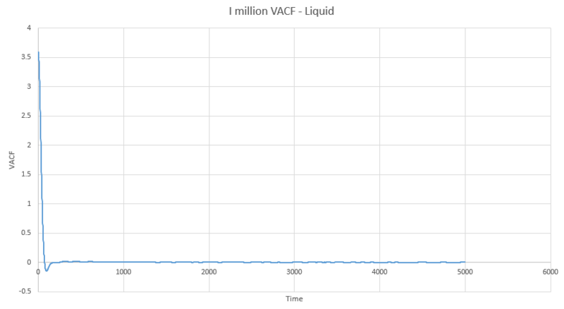
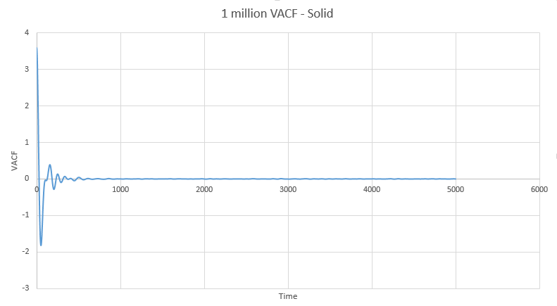
The full VACF plots for solid, liquid and vapour from the simulations run are below:

TASK: Use the trapezium rule to approximate the integral under the velocity autocorrelation function for the solid, liquid, and gas, and use these values to estimate $D$ in each case. You should make a plot of the running integral in each case. Are they as you expect? Repeat this procedure for the VACF data that you were given from the one million atom simulations. What do you think is the largest source of error in your estimates of D from the VACF?

To be able to calculate the diffusion coefficients using the VACF, the integral must be estimated using the trapezium rule which takes the form: (h/2)[f(x₀) + 2f(x₁) + 2f(x₂) + ... +2f(x_n-1) + f(x_n)] where h is the width of the interval and the x₀, x₁, etc., are the points at the beginning and end of each interval.

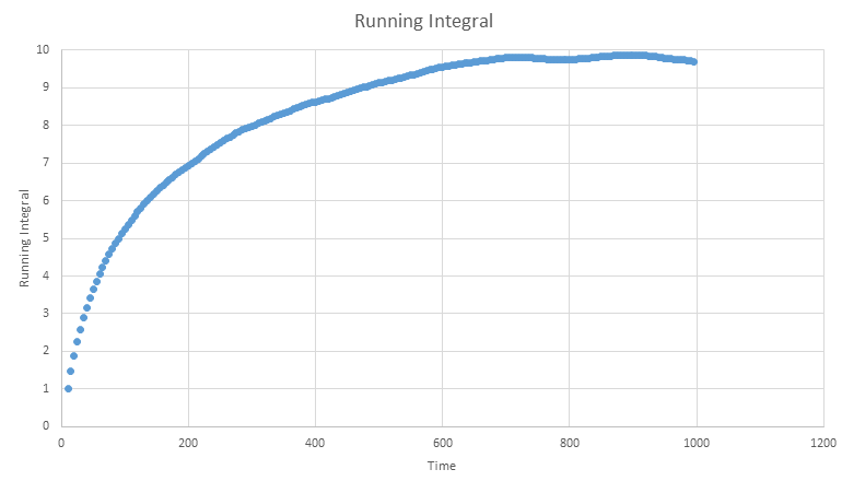
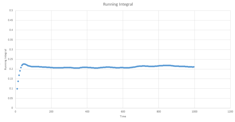
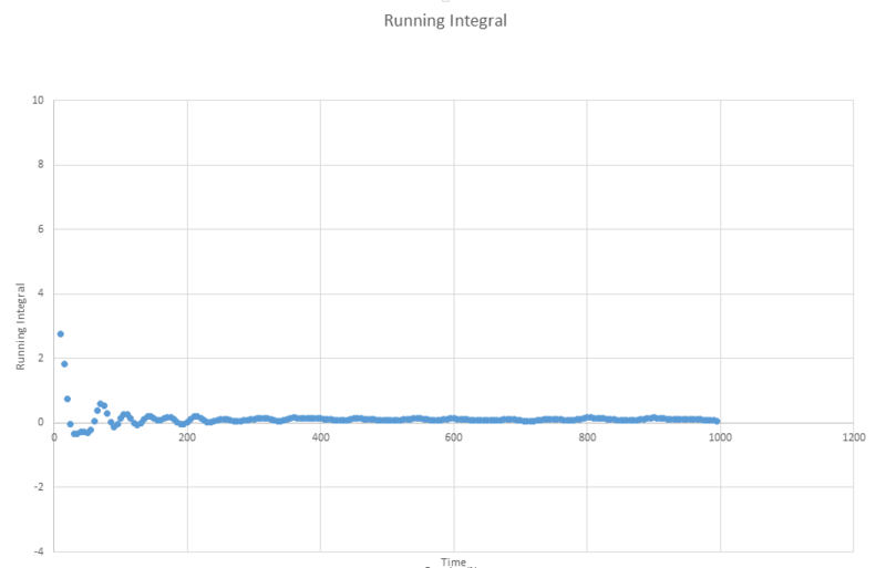
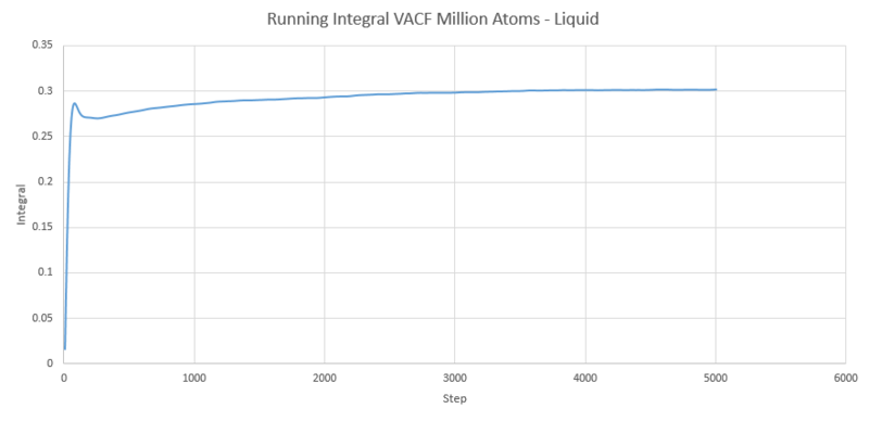
Below the running integrals for the simulated VACF functions are shown, these were obtained by implementing the trapezium rule as described above then diving the final result by three.

Gas: D = 3.21616

Liquid: D =0.806504

Solid: D = 5.68x10^-4

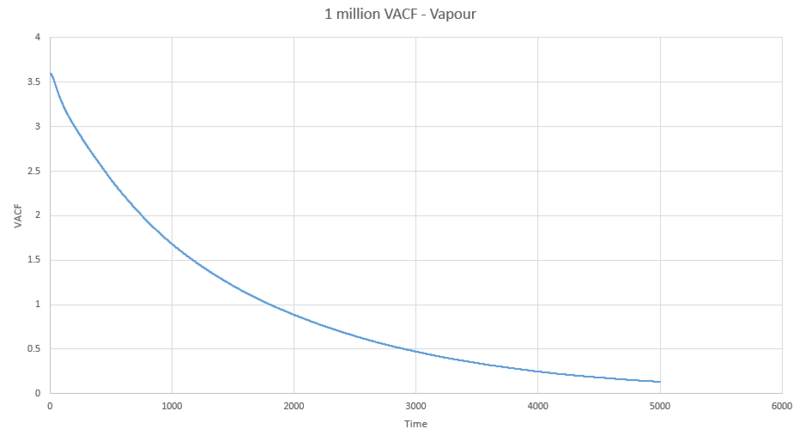
The next three plots were made following the same procedure as the previous three plots and the D values obtained in the same way but these are for the one million atom VACF simulations. The VACF plots are shown first, followed by the corresponding running integral.

Gas: D = 3.99689

Liquid: D = 0.103259

Solid: D = 3.46x10^-5

The running integral plots are not surprising given the shape of the plots of VACF as we know that we see a large under-curve area at lower time which damps down to zero as time increases. The D values we get out are shifted a few orders of magnitude to those gained from using the mean squared displacement however the established trend is still as we expect and there is some inherent error in using the trapesium rule as it is always just and estimate to the true value of the integral. However, this is not the main source of error when calculating the diffusion coefficient in this way. We see in the plots of VACF a fairly rapid decay to values nearing zero, however the tail off to reach a zero value can be very long and so integration over shorter time periods can lead to vast underestimates in the value of D. As we can see our D values are significant underestimates if taken with respect to the MSD calculated values, which only depend on the slope and so we do not need such long range time to establish an accurate value for D. NJ: the discrepancy is actually more because the units of D from the MSD are wrong. If you multiply them by about 1000 (same order as multiplying by the timestep), they're much more comparable. A table to compare the 12 different D values that you obtained would be good (and also an indication of the density and temperature of the states that you simulated).